
1.1 Purpose
The pest control industry experienced steady top-line growth between 2023 and 2025. However, growth alone did not guarantee stronger profitability. Labor costs, indirect overhead, vehicle expenses, and growth-related investments have shifted differently across operators and company sizes. As a result, profitability increasingly depends not just on growth, but on how effectively operators manage their cost structure as they scale.
This study examines where profitability pressure is building within the pest control industry and how those pressures vary by revenue tier and operating model. By comparing performance across segmented peer groups, the benchmarks in this report help operators see where their business stands relative to industry norms and identify the operational drivers most responsible for Margin pressure.
Rather than relying on simple averages, the analysis focuses on performance distributions, highlighting the gap between median performance and best-quartile execution. Segmenting operators by revenue tier and region enables more meaningful comparisons that reflect differences in scale, labor markets, and operating environments. For example, operators generating less than $1M in revenue often face fundamentally different operational constraints than companies operating above $3M in annual revenue, where staffing structures, overhead allocation, and growth investments tend to evolve significantly.
The objective is not simply to measure performance, but to clarify the structural factors separating disciplined operators from those experiencing Margin compression heading into 2026. The analysis also highlights how operators achieving both strong growth and strong Margins manage these pressures differently, offering practical insights for businesses seeking to improve profitability without sacrificing growth.
FRAXN's role is to translate financial data into clear, consistent reporting structures that reflect how the business has actually performed. This includes analyzing what the levers behind those numbers are, identifying where performance is stable or volatile, and clarifying what the data supports today. The objective is not to prescribe actions, but to make the financials transparent and defensible so operators can make informed decisions grounded in reality.
1.2 Who Should Read This Report
This study is most relevant for decision-makers within pest control organizations, including:
- Owners and founder-operators
- General managers and COOs
- CFOs and finance leaders
- Growth-focused operators evaluating operational scalability
- Investors and strategic partners (secondary audience)
The analysis is particularly useful for operators seeking to:
- Benchmark cost structure against similarly sized peers
- Diagnose Margin compression despite Revenue Growth
- Evaluate whether growth investment is translating into profitable expansion
- Inform 2026 planning with realistic, scale-adjusted financial guardrails
- This report is not intended as a general industry overview. It is a structural benchmarking study designed for operators actively managing cost discipline, growth quality, and long-term profitability.
1.3 What Makes This Study Different
Unlike traditional industry surveys that rely on blended averages, this study emphasizes structural dispersion, meaningful segmentation, and multi-year performance trends.
Key differentiators include:
- Segmentation FirstBenchmarks are presented by revenue tier and region, avoiding blended averages that can obscure the operational dynamics of scale.
- Multi-Year PerspectiveLeveraging full-year financial data from 60 operators, the study provides a multi-year comparison spanning 2023–2025, highlighting how performance patterns evolve over time.
- Distribution-Based MetricsResults are reported using medians and quartile ranges rather than simple averages. This approach reduces distortion from outliers and provides a clearer picture of typical operator performance.
- Dynamic Performance AnalysisBeyond static benchmarks, the study introduces performance relationship analysis, examining how key variables interact rather than viewing them in isolation. Visual analyses such as Revenue Growth versus expense expansion, growth versus Margin change, and investment intensity versus profitability highlight the structural trade-offs operators face when scaling. These relationship-based insights reveal patterns that traditional quartile tables alone cannot capture.
- Growth Quality FrameworkThe study evaluates not only how fast operators grow, but also how efficiently they grow. By examining how expenses scale relative to revenue, the analysis links cost behavior directly to EBITDA outcomes. This approach helps operators understand not just where they stand, but why performance differs across the industry and how those differences evolve over time.
tldr; Chapter 1 — Report Positioning
Summary Points
- This report exists because revenue growth alone doesn't tell you enough.Between 2023 and 2025, most pest control operators grew. But labor costs, indirect overhead, and vehicle expenses quietly eroded margins for many of them. Knowing your revenue number is not the same as knowing how your business is actually performing.
- The data comes from real financials, not surveys.Every figure in this study is drawn from actual bookkeeping records, standardized into a consistent framework across 125 operators. That is what makes it useful. Industry surveys measure what operators believe. This report measures what their books actually show.
- The goal is practical, not academic.This report is designed to answer four questions: Where is margin pressure building? How does your performance compare to peers? Which cost drivers separate disciplined operators from the rest? And what financial guardrails should shape your 2026 planning?
- This report is for you if you have ever looked at your P&L and thought, "I'm not sure if this is good or not."Whether you grew and want to know if your margins kept pace, or you're preparing for 2026 and want data-backed benchmarks, this report was built to answer those questions with real numbers, not industry generalizations.
- How to use it: find your tier, match your region, compare to median and top quartile.Use your 2025 revenue to identify your tier (under $1M, $1M to $3M, $3M+). Reference your region for additional context. Then focus on the largest gap between your numbers and the top quartile, and start there.
- Median is not the goal. Understanding why the gap exists is.The most valuable part of benchmarking is not the number itself. It is the question it forces: why does my business look different from the most disciplined operators, and what cost decisions are driving that difference?
See How Your Numbers Compare
Every benchmark in this report can be applied directly to your own P&L. If you want to know exactly where your business stands, FRAXN works with pest control operators to build the financial clarity this report measures. Visit fraxn.com or scan the QR code to learn more.


2.1 Data Source and Standardization
This study is built from operator-level financial data provided by participating pest control companies. To ensure comparability across businesses with different bookkeeping practices, financial entries were standardized into a consistent chart-of-accounts (COA) structure, enabling true apples-to-apples benchmarking.
Because accounting treatment varies across operators, particularly for subcontracted labor, fleet costs, and employee-related expenses, accounts are mapped based on economic function rather than company-specific chart-of-accounts structures. For example, indirect payroll is separated to exclude compensation attributable to Sales and Marketing activities when those costs are recorded within broader payroll accounts. This ensures benchmarks reflect operational reality rather than accounting classification differences.
2.2 Cohort Definition
Two cohorts are referenced throughout this study:
- Cohort A (3-Year Trend Cohort):Operators with complete financial data for 2023–2025 (n = 60). This cohort is used exclusively for multi-year trend analysis and volatility insights. It represents a subset of the broader benchmark sample.
- Cohort B (Benchmark Cohort):Operators with complete financial data for 2024–2025 (n = 125) comprise the primary benchmarking cohort used for cost structure analysis, segmentation, growth comparisons, and profitability evaluation. Within this group, nine operators began operations partway through 2024. Although these companies report financial data for both years, their 2024 results do not represent a full operating period.
To preserve true comparability and avoid distortion from partial-year ramp-up effects, FRAXN did not annualize their 2024 financial records to account for missing months. Where full-year comparability is required for 2024–2025 analysis, the study uses a subset of operators with complete operating periods, referred to as the comparable cohort (n = 116). The full benchmark cohort (n = 125) is retained for structural benchmarking analyses. Unless otherwise noted, all structural benchmarking results reference Cohort B (n = 125).
2.3 Chart of Accounts to Benchmark Mapping
Each operator's financials have been translated into FRAXN's uniform chart of accounts providing a standardized benchmarking framework. A full chart-of-accounts (COA) mapping used in this study is provided in the Appendix for reference.
The guiding principle is straightforward:
- Cost of Service (COS)reflects what it takes to perform the work.
- Operating Expense (OPEX)reflects what it takes to run and grow the company.
Unless otherwise noted, benchmarks are expressed as a percentage of revenue for the applicable year of analysis.
Year-over-year changes in cost structure are measured as percentage-point (pp) differences relative to revenue, not as dollar growth rates. For example, if Cost of Service increases from 45% of revenue in 2024 to 48% in 2025, the change is reported as a +3 percentage-point increase, meaning $0.48 of every revenue dollar is now spent performing the work, compared with $0.45 the prior year.
Comparative revenue tiers are based on 2024 baseline revenue and remain fixed across the 2023–2024 and 2024–2025 comparisons to avoid artificial tier migration.
2.4 Benchmark Statistics and Weighting
All published benchmarks use company-weighted distribution statistics:
- Median (50th percentile)
- Best Quartile (75th or 25th percentile depending on the benchmarking metric)
Company-weighted means each operator contributes equally to the distribution, regardless of company size or revenue scale.
Because benchmarks rely on medians and quartiles rather than arithmetic averages, extreme values have reduced influence on the published statistics. Observations are retained unless a clear data integrity issue is identified.
Distribution statistics are used instead of revenue-weighted averages to preserve comparability across operators of different sizes and operating scales.
How to Read the Benchmark Charts (Boxplots)
The charts in this report visualize distribution statistics using boxplots, showing how performance varies across operators.
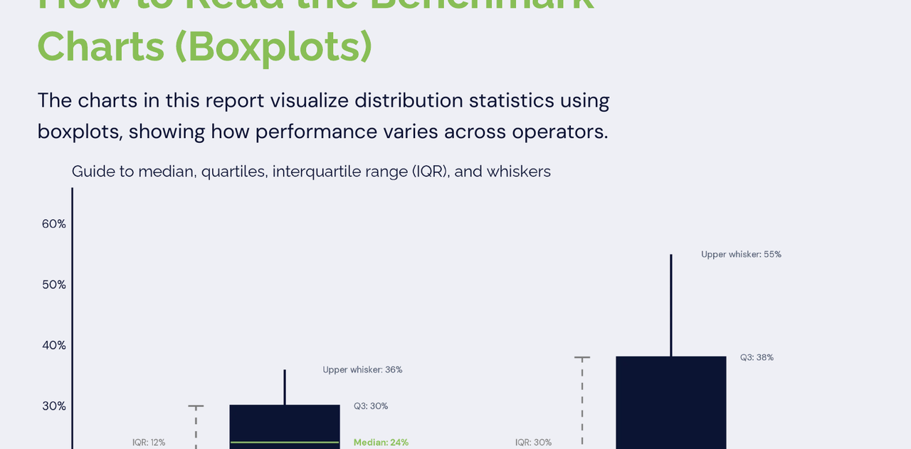
Each boxplot summarizes the distribution:
- The horizontal line inside the box represents the median, which is the typical operator performance.
- The box shows the distribution of the middle 50% of operators. Where the upper edge represents the Q3 (75th percentile) while the lower edge represents Q1 (25th percentile).
- The height of the box (IQR) reflects how consistent or variable the results of the middle 50% are across peers.
- The whiskers show how far results extend beyond the middle 50% of operators, indicating the wider range of outcomes in the dataset.
How to interpret the Distribution:
The example chart above illustrates how distributions can differ even when medians are similar.
- In the tighter spread example, results are more consistent:
- Median: 24%
- Most operators fall within a narrow range (18% to 30%)
- The IQR is relatively small (12 percentage points gap)
- In the wider spread example, performance varies significantly:
- Median: 22% (similar to the first example)
- However, results range much more widely (6% to 38% within the box)
- The IQR spreads to 30 percentage points, indicating higher variability
Despite having similar median values, the second group shows much greater dispersion, meaning operator performance is less consistent and more diverse. On this example you can initially ask the "Same median = same performance environment".
How to Benchmark Yourself
Use each chart to assess your position:
- At the median = You are in line with the typical operator
- Above or below the median = You are outperforming or lagging peers
- Outside the box (above Q3 or below Q1) = You are materially different from the market
- Within the box = You are operating within the typical range
Interpreting "Best Quartile"
"Best" performance depends on the metric:
- Growth and profitability metrics → Higher is better (top quartile / Q3)
- Expense metrics → Lower is better (bottom quartile / Q1)
What to Focus On
When reviewing benchmarks, focus on:
- Your distance from the median
- The spread of the distribution (tight vs wide)
- Which cost or revenue drivers explain the gap
Benchmarking your operating figures shows where you stand while the distribution shows how competitive that position really is.
2.5 Metric Construction — Core Benchmark KPIs
Profitability in this report is evaluated through a sequential operating structure that reflects how revenue converts into operating profit. The benchmarks follow a simple progression:
Revenue → Cost of Service → Gross Margin →
→ Operating Expenses → EBITDA Margin %
This structure isolates where Margin pressure originates, whether within service delivery or within broader operating overhead.
Revenue and Profitability Benchmarks
The following metrics capture the primary performance outcomes of pest control operators, including Revenue Growth, Gross Margin, and operating profitability. These benchmarks reflect how effectively operators convert revenue into profit across different cost structures and operating models.
Revenue Growth %
(Current Year Revenue − Prior Year Revenue) ÷ Prior Year Revenue
Measures year-over-year change in total revenue relative to the prior-year baseline. Revenue Growth reflects the pace at which operators expand through customer acquisition, pricing adjustments, and service volume.
Gross Margin %
(Revenue − Cost of Service) ÷ Revenue
Measures the portion of revenue remaining after direct service delivery costs are deducted.
Gross Margin provides an indicator of field-level operating efficiency before administrative overhead and growth investments are considered. It helps determine whether Margin pressure originates within service delivery or elsewhere in the cost structure.
EBITDA Margin %
(Revenue − Cost of Service − Operating Expenses) ÷ Revenue
Measures overall operating profitability after both service delivery costs and operating overhead are deducted.
For benchmarking consistency, accounts related to financing activities, income taxes, and other non-operating items are excluded from the analysis.
Because depreciation, amortization, and certain non-operating accounts are not consistently reported across operators, EBITDA in this study should be interpreted as an operating profitability benchmark rather than a strict accounting EBITDA measure.
This standardized definition provides a consistent basis for comparison across operators regardless of capital structure, ownership, or accounting treatment.
Cost Benchmarks
The following metrics decompose the operating cost structure underlying Gross Margin and operating profitability. Evaluating each component individually reveals the cost drivers behind the performance benchmarks.
Cost of Service (COS) %
Cost of Service ÷ Revenue
Cost of Service includes only direct costs required to deliver pest control services, including:
- Direct Field Labor ExpenseIncludes Payroll, payroll taxes, benefits, and subcontractor payments for technicians and other personnel directly performing field service work.
- Materials, Chemicals & Small Equipment Expenseincludes operating inputs directly consumed in the delivery of pest control services, including chemicals and treatment products; baits, traps, and other consumable supplies; small tools and service equipment purchases; equipment leases directly tied to field operations; and field uniforms and related service gear.
- Direct Field Vehicle / Fleet Expenseincludes fleet-related costs directly tied to service delivery, such as fuel, lease, repairs, maintenance, insurance and other vehicle expenses.
Note: Where operators record vehicle costs across multiple accounts, expenses are mapped based on their economic function to ensure costs associated with field service delivery are consistently included in Cost of Service.
- Other Direct Costincludes other expenses that are directly attributable to performing field work.
Operating Expenses (OPEX) %
Operating Expenses ÷ Revenue
Operating Expenses represent all indirect costs required to support the business beyond direct service delivery.
OPEX is not benchmarked as a single aggregate percentage in this study. Instead, analysis is performed at the component level to improve diagnostic precision and allow operators to isolate specific cost drivers rather than reacting to blended overhead totals.
Primary OPEX components include:
- Indirect Labor Expenseincludes personnel-related expenses for non-field roles that support operations, administration, and management functions.
Note: Where payroll accounts combine multiple functions, compensation is reclassified based on job function to ensure administrative labor is separated from field labor and Sales & Marketing activities.
- Sales & Marketingincludes all payroll and non-payroll expenses directly associated with customer acquisition, promotion, and revenue generation. Sales & Marketing % reflects customer acquisition intensity and growth investment level. It should be evaluated alongside Revenue Growth %, Gross Margin %, and payback metrics when assessing growth efficiency.
Note: Where sales-related payroll or marketing expenses are embedded within broader payroll or administrative accounts, costs are mapped to Sales & Marketing based on their underlying economic function.
- Facility / Occupancyincludes all costs associated with maintaining office, warehouse, and operational premises, as well as supporting communication and office infrastructure.
- G&Aincludes corporate-level administrative, financial, compliance, insurance, professional service, and general business expenses required to manage and govern the company that are not directly tied to service delivery, fleet operations, sales and marketing, or facility infrastructure.
- Other Indirect Costincludes other expenses required to support the business beyond direct service delivery.
Note on Interpretation: All cost metrics are expressed as a percentage of revenue at the company level and summarized using the median across operators. Because each component is calculated and aggregated independently, the sum of median cost components will not equal total Cost of Service or Operating Expenses and will not reconcile to 100%.
This approach is intentional and provides a more accurate view of typical cost allocation across operators, avoiding distortion from outliers or differences in company size.
2.6 Segmentation Approach
Benchmarks are segmented to avoid blended averages that may obscure scale effects.
Primary segmentation: Revenue Tier (based on annualized revenue)
After careful consideration and participant analysis, FRAXN categorized participants into three revenue segments based on their annualized revenue.
- Less than $1M (<$1M)Those operators with less than $1M annualized revenue.
- $1M to $3M ($1M−$3M)Those operators with revenues between $1M and $3M annualized revenue.
- Greater than $3M ($3M+)Those operators with revenue greater than $3M annualized revenue.
For a more detailed overview of participant distribution by Revenue Tiers, please refer to Chapter 4.2 Revenue Tier Distribution.
Secondary segmentation: Region (where sample sizes support meaningful comparison)
Operators should benchmark primarily against their revenue tier and then reference regional comparisons where applicable.
The regions included in this report are:
Mid-Atlantic North Central North East Pacific North West
South Central South East South West
For a more detailed overview of participant distribution by Region, including state-level representation, please refer to Chapter 4.3 Geographic Representation.
2.7 Data Limitations
Regional Coverage
Cohort A (2023–2025 trend cohort) has limited participation in certain regions. No North Central operators currently meet full three-year data requirements. As a result, three-year trend analysis for that region is not presented.
In regions with smaller sample sizes, benchmark results should be interpreted with appropriate caution, as thinner cohorts may be more sensitive to the performance of a small number of operators. As participation expands over time, regional benchmarks are expected to become more stable and representative.
Scale Sensitivity in <$1M Tier
Within the <$1M revenue tier, percentage changes in growth and Margin metrics may appear amplified due to smaller revenue bases. These observations are retained in the dataset. However, the use of company-weighted medians and quartiles reduces the influence of extreme values. Results should be interpreted with appropriate consideration of scale sensitivity.
Source Data Treatment
Financial data used in this study is derived from a combination of operator-submitted bookkeeping records and FRAXN-managed accounting records. While FRAXN standardizes accounts into a consistent benchmarking framework, underlying transaction classification generally follows each participating company's internal reporting practices.
FRAXN performs structural mapping to a standardized chart-of-accounts to ensure comparability across operators. However, no forensic reclassification, audit procedures, or reconstruction of financial statements were performed beyond this standardization process.
As a result, the benchmarks presented in this report reflect reported operating performance rather than audited or restated financial results.
Treatment of Negative Category Totals
Negative totals within Cost of Service (COS) or Operating Expense (OPEX) categories may occur due to accounting reversals, reclassifications, or one-time adjustments. Immaterial negative amounts are retained. Where negative category totals exceed a materiality threshold (e.g., 1% of revenue), they are capped at zero for benchmarking ratio calculations to preserve structural comparability across operators.
Visualization Adjustments
In certain visualizations, particularly scatter plots, extreme outlier observations may be omitted from the chart display to improve readability and highlight the primary distribution of results. These extreme cases represent a very small number of observations and do not materially affect the underlying benchmark calculations.
Unless otherwise noted, distribution statistics and benchmark values are calculated using the full dataset, with observations retained unless a clear data integrity issue is identified.
Go-to-Market Model Differences (D2D / High Acquisition Spend)
Some operators utilize door-to-door (D2D) or other high-investment sales models, which structurally increase sales payroll and marketing expense relative to peers. Benchmark comparisons should account for differences in go-to-market strategy, customer acquisition intensity, and service mix when interpreting cost structure and Margin outcomes. Results should be interpreted with appropriate consideration of this business model differences.
tldr; Chapter 2 — Data, Cohorts, and Methodology
Summary Points
- Two cohorts. One for benchmarking, one for trends. Cohort B is 125 operators with complete 2024 and 2025 financials, used for all primary benchmarks. Cohort A is a 60-operator subset with three full years of data (2023 to 2025), used exclusively for multi-year trend analysis. These are not interchangeable.
- Every operator's financials were standardized before any comparison was made. Businesses with different bookkeeping practices, account structures, and expense classifications are translated into a consistent chart of accounts before a single benchmark is calculated. This is what makes the numbers comparable.
- Cost of Service covers what it takes to perform the work. Direct Field Labor, materials and chemicals, and field vehicles. Operating Expenses cover what it takes to run and grow the company: indirect labor, Sales and Marketing, facility costs, and G&A. Understanding which side of that line your costs live on is the foundation of this entire analysis.
- Medians and quartile ranges, not averages. This prevents a handful of unusually large or small operators from skewing the results. Every operator contributes equally to the distribution regardless of company size. When you see a benchmark number in this report, it represents the typical operator, not an outlier-influenced mean.
- Benchmarks are segmented by revenue tier and region. Comparing a $500K operator to a $5M operator produces noise, not insight. Tier and region segmentation ensures you are always looking at peers operating under similar conditions. Always use your revenue tier before layering in regional context.
- Door-to-door and high-acquisition models will look different. If your go-to-market relies on D2D sales or aggressive acquisition spend, your Sales and Marketing costs will structurally sit above the benchmark median. That is not a red flag. It reflects a deliberate strategy, and the report accounts for that distinction.
- The data reflects reported operating performance, not audited financials. Accounts are standardized for comparability. They are not reconstructed or restated. That distinction matters when interpreting any benchmark figure and is documented in full in the methodology appendix.

Industry Performance Snapshot
This benchmark study analyzes financial performance across 125 pest control operators, with 116 companies forming the comparable cohort used for growth and profitability analysis between 2024 and 2025. Participating operators span multiple revenue tiers and geographic regions, providing a broad view of the economic structure of modern pest control businesses.
At a structural level, the economics of pest-control operators demonstrates a consistent, cost-intensive model across all revenue tiers.
Across the benchmark cohort:
- Cost of Service represents approximately 35–40% of revenue
- Operating Expenses account for roughly 44–46% of revenue
- Resulting in median EBITDA Margins of 15–17%
While larger operators benefit from higher Gross Margins, this advantage is partially offset by higher overhead requirements, resulting in relatively similar EBITDA Margins across tiers. This highlights that scale alone does not guarantee improved profitability and cost discipline remains critical at all levels.
Overall, the industry continues to demonstrate strong expansion. Median Revenue Growth reached 15.4%, with the middle 50% of operators growing between 5.7% and 28.9%. This reflects sustained demand for recurring pest management services and continued expansion across many operators.
However, Revenue Growth did not consistently translate into stronger profitability. For many operators, expenses increased at a similar or faster rate than revenue, limiting Margin expansion.
These findings indicate that the next phase of industry performance will depend less on pure Revenue Growth and more on how effectively operators manage cost components such as labor productivity, marketing efficiency, and overhead structure as they scale.
Growth Remains Strong, but Expenses Are Expanding at Similar Rates
A consistent pattern across the study is the close relationship between Revenue Growth and Expense Growth.
Many operators cluster near the diagonal line, where revenue and expenses are growing at similar rates. Points above this line represent companies whose total costs and expenses are rising faster than revenue, placing pressure on margins. Points below the line indicate operators that are successfully capturing operating leverage, where revenue growth outpaces growth in costs and expenses. Of the 116 operators analyzed, 56 experienced Expense Growth outpacing revenue, while 60 achieved Revenue Growth ahead of expenses, representing a near-even split between less efficient and more efficient growth outcomes.
While some companies achieved strong growth alongside improving margins, the broader distribution shows that growth alone does not guarantee stronger profitability. Expansion often requires reinvestment in technician capacity, marketing, and operational infrastructure. Operators that convert growth into margin improvement tend to maintain discipline in staffing, route density, and marketing efficiency.
Efficient Growth Is Not Universal
The relationship between Revenue Growth and Margin change reveals four distinct operating profiles among the 116 operators with full-year comparability.
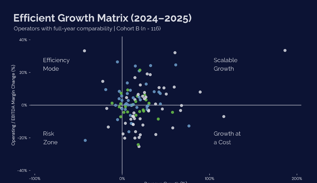
| Quadrant | Operators (n) | Share of Sample | Median Revenue Growth | Median EBITDA Margin Change |
|---|---|---|---|---|
| Scalable Growth | 49 | 42% | 23.4% | +7.1% |
| Growth at a Cost | 47 | 41% | 16.8% | -6.8% |
| Efficiency Mode | 11 | 9% | -3.5% | +7.3% |
| Risk Zone | 9 | 8% | -5.2% | -2.2% |
- Scalable Growth | upper-right quadrant:Strong Revenue Growth with improving Margins
- Growth at a Cost | lower-right quadrant:Revenue Growth accompanied by Margin compression
- Efficiency Mode | upper-left quadrant:Stable profitability with slower growth
- Risk Zone | lower-left quadrant:Declining growth and Margins
The distribution across these profiles reinforces a key finding: efficient growth is not universal. While 42% of operators achieved both revenue expansion and margin improvement, nearly equally 41% grew revenue at the expense of maximized profitability.
Note: not all "Growth at a Cost" outcomes are equally negative. While 33 operators in this quadrant experienced a decline in absolute EBITDA dollar value, 14 operators (30%) still increased EBITDA despite margin compression. This indicates that in some cases, revenue growth was sufficient to offset declining margins, resulting in higher absolute profit even as efficiency weakened.
Only 17% of operators experienced revenue contraction, indicating that the industry broadly expanded during the period. Notably, over 80% of companies increased revenue, but nearly half did so without improving profitability.
What Separates Top Performers
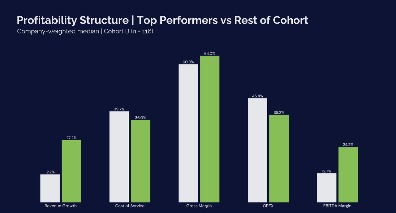
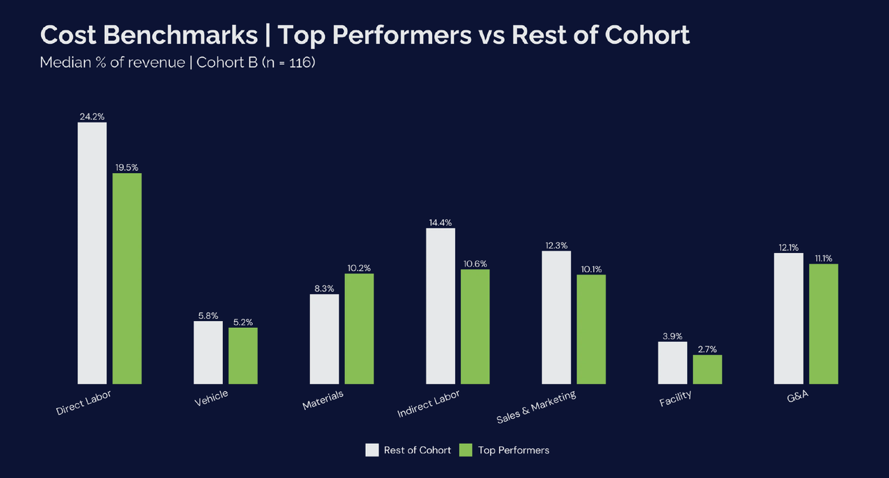
Operators achieving both above-median growth and profitability share several consistent characteristics.
Top performers maintain lower Cost of Service ratios, indicating stronger technician productivity and more efficient service delivery. They also operate with leaner staffing structures, resulting in lower overall people costs.
At a more diagnostic level, the cost structure reveals a clear pattern. Top performers maintain leaner benchmarks across all OPEX components. However, within Cost of Service, a different trend emerges. Top performers allocate a higher share of revenue to Materials, Chemicals, Equipment, and Field Supplies (10.2% vs 8.3%), signaling a deliberate investment in service quality rather than aggressive cost minimization. In the context of pest control, where outcomes are directly tied to treatment effectiveness, this higher spend likely supports better customer retention, fewer callbacks, and stronger recurring revenue streams.
Unlike labor or overhead, materials and equipment represent a critical input to service quality, not just a cost line to optimize. Underinvestment in chemicals or application equipment can compromise treatment effectiveness, leading to reduced customer satisfaction and higher churn, ultimately eroding long-term profitability.
Top performers demonstrate that growth and profitability are not mutually exclusive — they are the result of disciplined execution across labor, service delivery expenses, pricing, and operational structure.
Planning Implications for Operators
Several practical implications emerge from the benchmark analysis:
- Growth remains achievable but requires reinvestment Expansion typically requires increased spending in labor, marketing, and higher-quality service delivery inputs.
- Labor productivity is the primary profitability driver Improvements in technician efficiency and route density have a direct impact on Margins.
- Marketing effectiveness matters more than scale Successful operators focus on conversion and payback rather than increasing spend alone.
- Overhead discipline becomes critical at scale As companies grow, controlling administrative and support costs is essential to maintaining profitability.
tldr; Chapter 3 — Executive Summary
Summary Points
- The industry grew.Median Revenue Growth across 125 operators was 15.4% in 2025, with the middle 50% landing between 5.7% and 28.9%. Demand for pest control services remains strong and broadly distributed across regions and company sizes.
- Revenue growth did not reliably become profit.For many operators, expenses grew at roughly the same rate as revenue. The result: EBITDA Margins were essentially flat at the median, hovering between 15% and 17% across all revenue tiers.
- Scale did not solve the problem.Larger operators ($3M+) achieved higher Gross Margins from better route density and technician efficiency. Those gains were almost entirely offset by heavier overhead. Median EBITDA Margins were similar across every tier.
- Growth quality varied sharply.42% of operators achieved scalable growth (revenue up, margins up). 41% grew revenue while margins declined. Only 17% experienced any revenue contraction, meaning most of the industry is growing, but nearly half are growing at a cost.
- Top performers play a different game.Operators achieving both above-median growth and above-median profitability maintained lower labor costs, leaner overhead, and more efficient marketing. They also spent more on materials and chemicals, not less. Service quality drives retention.
- The next competitive edge is cost discipline.The pest control industry has captured the growth. The operators who build lasting businesses will be the ones who manage what it costs to deliver and support that growth.
Are You Growing Efficiently or Just Growing?
The benchmark shows clearly that revenue growth and profitability are two different things. FRAXN helps pest control operators track the metrics that answer that question every single month. Visit fraxn.com or scan the QR code to learn more.


4.1 Cohort Composition
The benchmark dataset (Cohort B) includes 125 operators with complete financial data for 2024–2025, forming the primary benchmarking cohort used throughout the study. Nine operators began reporting financial data mid-year in 2024. While these operators are included in the benchmark cohort for structural cost comparisons, they are excluded from 2024–2025 comparative analysis (n=116) to ensure full-year comparability. Revenue figures were not annualized to avoid distortion from ramp-up periods.
A subset of 60 operators with complete financial data from 2023–2025 (Cohort A) forms the trend cohort, which is used for multi-year growth and volatility analysis.
4.2 Revenue Tier Distribution
Operators are segmented into three revenue tiers, below is a snapshot of participating companies based on their 2025 annualized revenue:
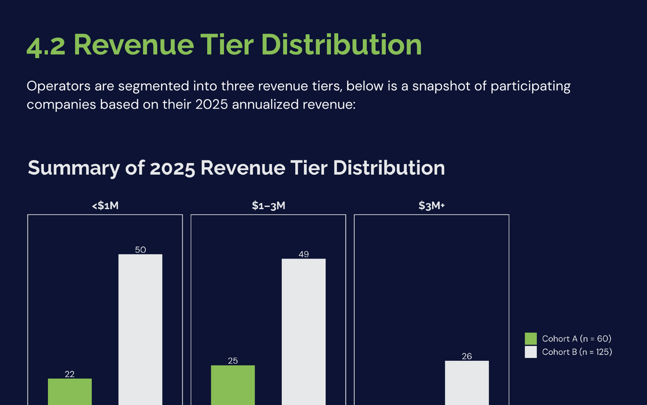
Benchmark tables use 2025 tier placement. Multi-year trend analysis uses a fixed baseline year 2024 to avoid artificial "tier jumping" caused by rapid growth.
Operators should first benchmark themselves against peers within the same revenue tier, as cost structure, staffing models, and overhead leverage tend to change materially as companies scale. Smaller operators typically rely on lean technician-driven operations, while larger operators often carry additional management layers, sales infrastructure, and administrative support. Comparing performance within similar revenue tiers helps ensure that benchmarking reflects structural differences rather than scale effects.
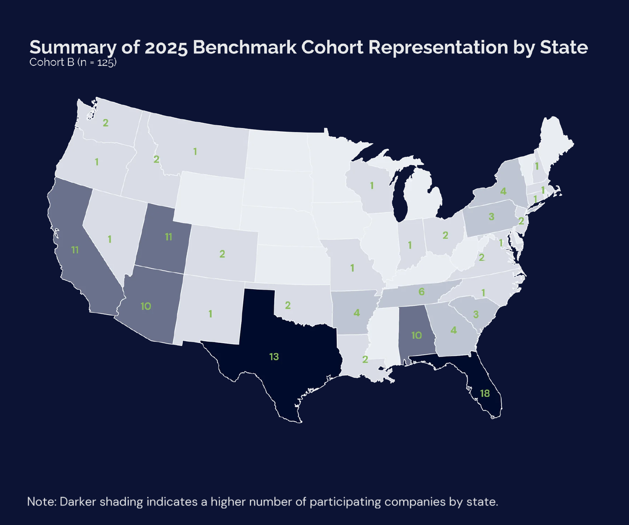
4.3 Geographic Representation
Participating operators span seven U.S. regions, providing broad geographic representation across diverse labor markets, service environments, and pricing conditions. In total, the benchmark cohort includes 125 companies distributed across these regions, with representation concentrated in the South East, South West, and South Central markets.
The regional composition and number of participating operators per state in this report is as follows:
- Mid-Atlantic (n = 10)Maryland (1), North Carolina (1), Tennessee (6), Virginia (2)
- North Central (n = 4)Indiana (1), Ohio (2), Wisconsin (1)
- North East (n = 12)Connecticut (1), Massachusetts (1), New Hampshire (1), New Jersey (2), New York (4), Pennsylvania (3)
- Pacific North West (n = 6)Idaho (2), Montana (1), Oregon (1), Washington (2)
- South Central (n = 25)Arkansas (4), Colorado (2), Louisiana (2), Missouri (1), New Mexico (1), Oklahoma (2), Texas (13)
- South East (n = 35)Alabama (10), Florida (18), Georgia (4), South Carolina (3)
- South West (n = 33)Arizona (10), California (11), Nevada (1), Utah (11)
Regional segmentation is applied where sample sizes support statistically meaningful comparisons, enabling operators to benchmark performance against peers operating under similar structural conditions.
The chart below summarizes regional participation across both cohorts, with 60 operators in the three-year trend cohort (Cohort A) and 125 operators in the benchmark cohort (Cohort B). Regions with smaller sample sizes, particularly North Central and Pacific North West, should be interpreted with appropriate caution, as results may be more sensitive to individual operator performance.
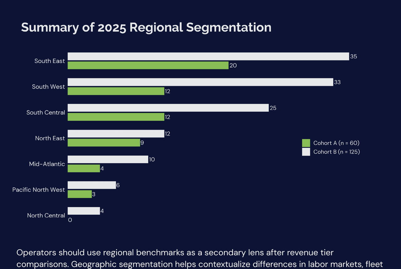
Operators should use regional benchmarks as a secondary lens after revenue tier comparisons. Geographic segmentation helps contextualize differences in labor markets, fleet operating costs, pricing dynamics, competition intensity, and service mix across regions. Benchmarking against peers operating in similar environments helps distinguish structural cost differences from internal operational inefficiencies.
tldr; Chapter 4 — Benchmark Dataset Overview
Summary Points
- 125 operators form the primary benchmark cohort. These are companies with complete financial data for 2024 and 2025. A separate 60-operator subset with three full years of data (2023 to 2025) is used exclusively for multi-year trend analysis.
- Revenue tiers reflect real operational differences. The three tiers (under $1M, $1M to $3M, $3M+) are not arbitrary groupings. Cost structure, staffing models, overhead leverage, and growth patterns change meaningfully as companies move between them. Always benchmark yourself against your own tier first.
- The dataset spans seven U.S. regions. Mid-Atlantic, North Central, North East, Pacific Northwest, South Central, South East, and South West. The South East (35 operators) and South West (33) carry the largest samples. North Central (4 operators) should be interpreted as directional, not definitive.
- Geography is a secondary lens, not the primary one. Use your revenue tier to establish your primary comparison. Then layer in regional benchmarks where they are relevant to your market conditions, labor costs, or pricing environment.
- This data was not self-reported. Unlike survey-based industry studies, these numbers come from actual bookkeeping records standardized by FRAXN before any comparison was made. That distinction matters when you are using the data to make real decisions.
Find Your Peer Group
Knowing your revenue tier and region is the starting point for benchmarking. FRAXN builds the financial infrastructure that makes this kind of comparison possible for individual operators. Visit fraxn.com or scan the QR code to get started.


Revenue growth, or top-line growth, is the starting point for evaluating operating performance and overall financial results. This chapter examines how operators expanded revenue from 2023 through 2025, first through a multi-year stability lens (Cohort A, n = 60), and then through the 2024–2025 comparable benchmark cohort (Cohort B, n = 116) to provide a clearer view of recent performance.
The objective is twofold: to assess growth consistency over time and to evaluate how current growth performance is distributed across comparable peers. All statistics are presented as company-weighted distributions.
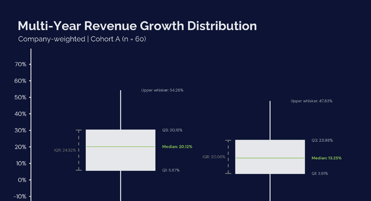
5.1 Multi-Year Growth Stability (2023–2025 | Cohort A n = 60)
To assess growth consistency and volatility, a subset of 60 operators with complete financial data from 2023 through 2025 was analyzed separately. Multi-year trend analysis uses this cohort only and should not be compared directly to the 125-company 2024–2025 benchmark dataset. Revenue tiers for multi-year analysis are fixed using 2024 baseline revenue to prevent tier shifting across years.
| Metrics | 2023→2024 | 2024→2025 | Description |
|---|---|---|---|
| Q1 (25th percentile) | 5.87% | 3.91% | Represents the lower quartile of Revenue Growth across operators for each period. |
| Median | 20.12% | 13.25% | Represents the typical Revenue Growth achieved by operators in each period. |
| Q3 (75th percentile) | 30.18% | 23.98% | Represents the upper quartile of Revenue Growth across operators for each period. |
| IQR (Q3–Q1) | 24.32 pp (percentage points) | 20.06 pp (percentage points) | Represents the spread between the 25th and 75th percentiles. |
This snapshot provides a benchmarking view of revenue growth stability across operators over the past two periods. While the interquartile range (Q3–Q1) indicates a relatively concentrated band of growth outcomes within the sample, the median growth rate declined from 20.12% in 2023–2024 to 13.25% in 2024–2025, a decrease of 6.87 percentage points (approximately 34%). This indicates that median revenue growth slowed materially between the two periods, reflecting a broad moderation in industry growth momentum rather than isolated underperformance.
The elevated growth environment in 2023–2024 also created conditions where operational inefficiencies could be masked or overlooked, as strong top-line expansion offset underlying cost pressures. As growth normalizes in 2024–2025, these inefficiencies become more visible, placing greater emphasis on cost structures and operating discipline.
As growth rates normalize, operators can no longer rely on top-line expansion alone to sustain profitability. Businesses built around aggressive growth capital deployment may begin to experience margin pressure as revenue expansion slows while cost structures remain elevated.
Operators should evaluate whether their current cost structure, staffing levels, and growth investments remain appropriate under a slower growth environment, and identify where operational efficiency or pricing adjustments may be required to maintain profitability.
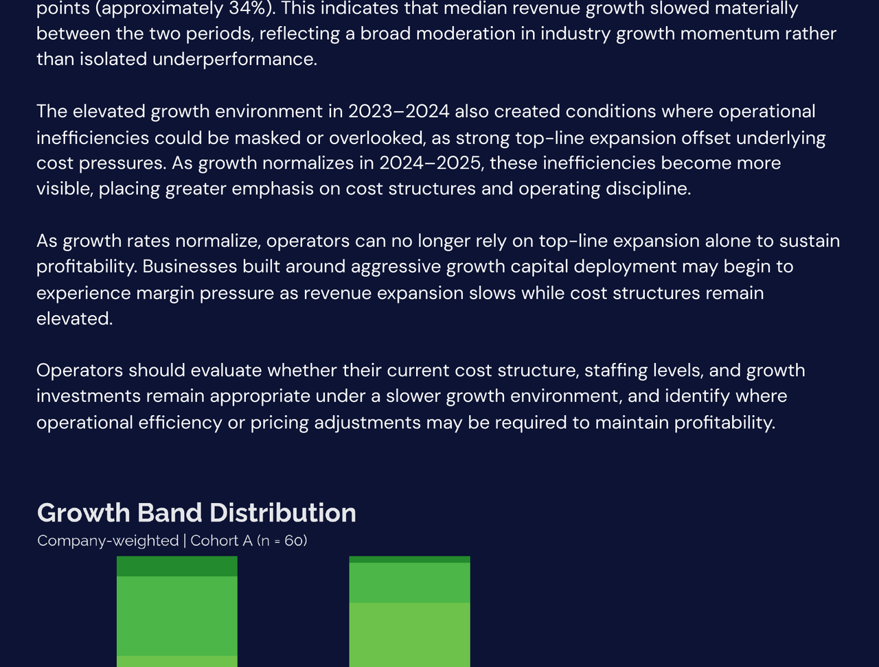
| Category | 2023→2024 Companies (%/n) | 2024→2025 Companies (%/n) | Description |
|---|---|---|---|
| Hyper Growth (≥ 100%) | 5.00% (3) | 1.67% (1) | A small subset of operators experiencing exceptionally rapid revenue growth, typically associated with acquisitions or major scaling events. |
| Large Growth (≥ 30% and < 100%) | 20.00% (12) | 10.00% (6) | Operators delivering strong revenue expansion, often reflecting accelerated customer acquisition, new service lines, or market expansion. |
| Growing (≥ 0% and < 30%) | 58.33% (35) | 65.00% (39) | Represents majority of the operators achieving steady year-over-year revenue growth. |
| Declining (> -15% and < 0%) | 15.00% (9) | 15.00% (9) | Operators reporting moderate declines in revenue during the period. |
| Underperforming (≤ -15%) | 1.67% (1) | 8.33% (5) | Operators experienced significant revenue contraction year-over-year. |
The growth band distribution provides a benchmark view of how revenue expansion is distributed across operators over the two-year period.
Most companies have steady growth band (0–30%), indicating that moderate, consistent expansion represents the typical growth pattern in the industry.
However, the data also shows a noticeable shift between periods, with the share of operators experiencing significant contraction increasing from 1.67% in 2023–2024 to 8.33% in 2024–2025, while the proportion of companies achieving large or hyper growth declined.
These patterns signal that while growth remains common across the cohort, outcomes are becoming more uneven and moderating in recent years, reinforcing the need to benchmark performance and establish clear guardrails to peers, rather than relying solely on top-line growth.
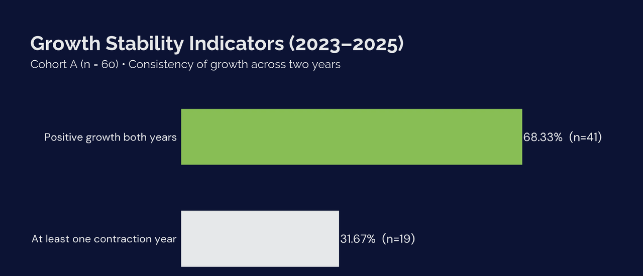
| Stability Metric | % of Companies | Operators (n) | Description |
|---|---|---|---|
| Positive growth both years | 68.33% | 41 | Operators that achieved revenue growth in both periods (2023–2024 and 2024–2025), indicating sustained expansion across the two-year window. |
| At least one contraction year | 31.67% | 19 | Operators that experienced a revenue decline in at least one of the two periods, reflecting some degree of growth volatility. |
| Declined both years | 8.33% | 5 | Operators that reported revenue contraction in both periods, indicating persistent negative growth over the two-year window. This is a subset of operators that experienced at least one contraction year. |
While industry expansion remains structurally intact, growth rates appear to be moderating. Approximately 68% of operators generated positive Revenue Growth in both periods, indicating sustained expansion across much of the sample. However, nearly one-third of companies experienced at least one contraction year. This pattern points out that growth stability is not universal across operators. Even within an expanding industry, individual operators may face volatility driven by local market conditions, customer churn, pricing pressure, or operational execution.
Operators should evaluate whether their growth model is resilient across multiple periods by examining customer retention, route density, and sales and marketing effectiveness to reduce the risk of intermittent revenue contraction.
5.2 Industry Growth Remains Positive but Performance is Fragmented
This section shifts from the multi-year cohort to the broader benchmark cohort to evaluate the most recent year-over-year performance from 2024 to 2025.
While the benchmark dataset includes 125 operators, nine companies began operations midway through 2024 and therefore do not reflect a full baseline year. To maintain comparability, FRAXN did not annualize partial-year revenue for these operators. As a result, the growth analysis for 2024–2025 reflects 116 operators with complete full-year data.
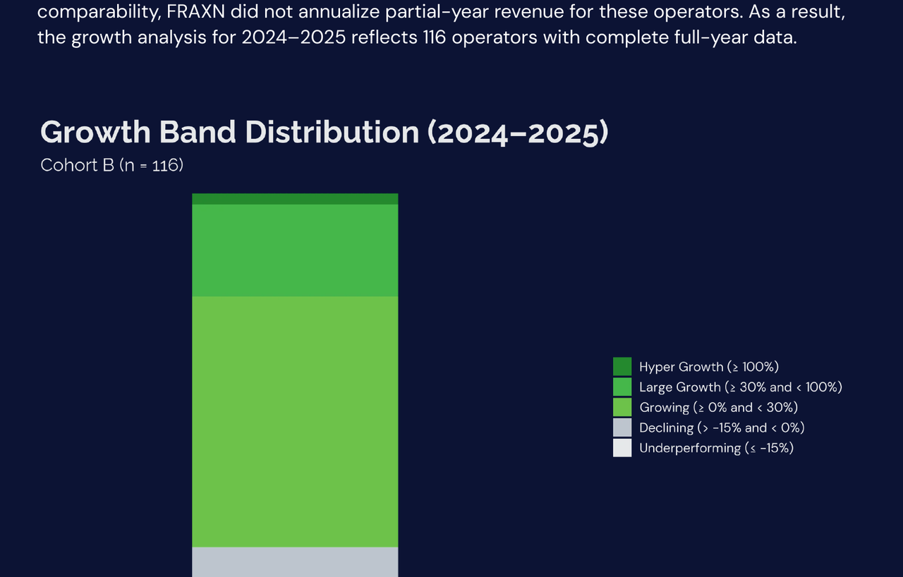
| Growth Band | % of Companies | Operators (n) | Description |
|---|---|---|---|
| Hyper Growth (≥ 100%) | 2.6% | 3 | A small subset of operators experiencing exceptionally rapid revenue growth, typically associated with acquisitions or major scaling events. |
| Large Growth (≥ 30% and < 100%) | 21.6% | 25 | Operators delivering strong revenue expansion, often reflecting accelerated customer acquisition, new service lines, or market expansion. |
| Growing (≥ 0% and < 30%) | 58.6% | 68 | Represents majority of the operators achieving steady year-over-year revenue growth. |
| Declining (> -15% and < 0%) | 12.1% | 14 | Operators reporting moderate revenue declines during the period. |
| Underperforming (≤ -15%) | 5.2% | 6 | Operators experiencing significant revenue contraction year-over-year. |
The findings across the benchmark group remain consistent. Revenue growth remained broadly positive, with approximately 83% of operators generating non-negative growth between 2024 and 2025 (Growing, Large Growth, and Hyper Growth), reinforcing the recurring revenue model that characterizes pest control services. The majority of operators (58.6%) fell within the moderate growth band of 0% to 30%, indicating that steady, incremental expansion remains the most common outcome across the industry.
However, performance outcomes are not uniform. While most operators grew, approximately 17.3% experienced some level of revenue contraction, including 5.2% with more pronounced declines. This variation highlights differences in execution, pricing power, service mix, and growth investment intensity across operators. Overall, the distribution suggests that growth is widespread but not evenly experienced, emphasizing that revenue expansion alone does not fully capture performance differences across the cohort.
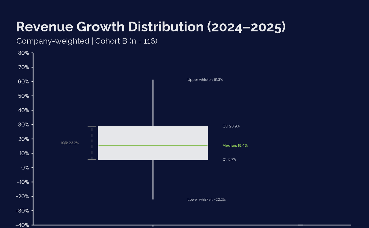
| Metric | Value |
|---|---|
| Q1 (25th percentile) | 5.7% |
| Median | 15.4% |
| Q3 (75th percentile) | 28.9% |
| IQR (Q3–Q1) | 23.2 pp |
Revenue expansion remains common across the industry, with the typical operator growing at 15.4% and most falling within a 5.7% to 28.9% range. This relatively wide middle band highlights that while growth is widespread, outcomes still vary meaningfully across operators. At the outer ends, a small number of companies experienced sharp contraction or outsized expansion, indicating that while extreme outcomes exist, they are not representative of the typical operator.
For this reason, growth should be viewed as a baseline rather than a signal of exceptional performance. Operators should assess performance relative to peers within their revenue tier, rather than relying on broad industry averages when identifying improvement opportunities.
5.3 Growth Diverges Materially by Revenue Tier
When segmented by revenue tier, growth outcomes diverge meaningfully across operators, indicating that scale influences both growth potential and volatility. Three structural distribution patterns emerge across the revenue tiers.
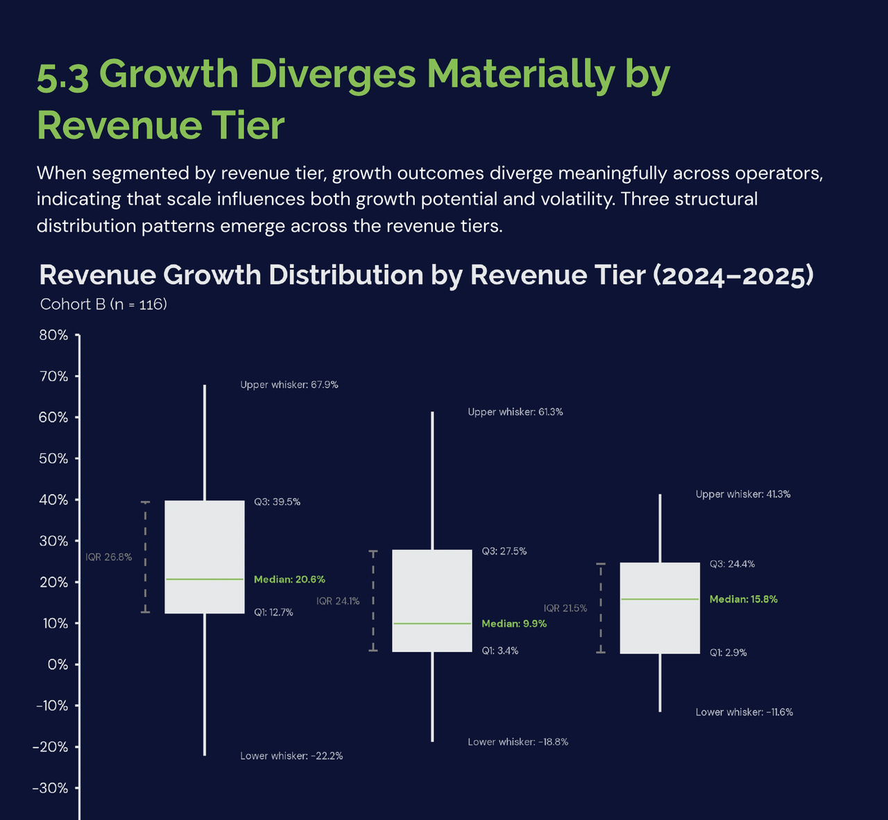
| Revenue Tier | Q1 (25th percentile) | Median | Q3 (75th percentile) | IQR (Q3–Q1) |
|---|---|---|---|---|
| <$1M | 12.7% | 20.6% | 39.5% | 26.8 pp |
| $1–3M | 3.4% | 9.9% | 27.5% | 24.1 pp |
| $3M+ | 2.9% | 15.8% | 24.4% | 21.5 pp |
<$1M — Rapid Expansion with Highest Variability
Smaller operators exhibit the fastest growth and the widest performance dispersion. Median growth reaches 20.6%, with upper-quartile outcomes approaching 40%, and the broadest interquartile range of 26.8 pp across tiers, highlighting the variability within this segment.
A meaningful portion of operators achieve very high growth rates, reflecting aggressive expansion from a smaller revenue baseline. At the same time, outcomes remain uneven as operators experiment with pricing strategies, marketing channels, and service mix.
This tier largely represents an expansion phase, where growth opportunities are abundant but operational structures are still developing.
$1–3M — The Structural Transition Zone
Growth moderates materially in the $1–3M segment. Median revenue growth declines to 9.9%, the slowest median outcome across all revenue tiers. While the typical operator performance in this segment continues to expand, the pace of growth becomes noticeably more constrained than in both smaller and larger peer groups. This pattern is consistent with the report's broader finding that the $1–3M range functions as a structural transition zone, where increasing organizational complexity begins to weigh on momentum.
At this stage, operators are often building the infrastructure required for the next phase of scale. Management layers begin to form, technician teams expand, and investment in sales and marketing becomes more formalized. These additions are necessary to support future growth, but they also introduce friction as costs and coordination requirements rise faster than the benefits of scale are fully realized.
In practical terms, the $1–3M tier represents an inflection point. Early-stage growth remains present, but it is no longer driven by lean, founder-led expansion alone. Operators that navigate this transition successfully are typically those that strengthen operating discipline while scaling, allowing systems, staffing, and revenue growth to mature in step rather than fall out of balance.
$3M+ — Stabilization and Operational Discipline
Larger operators demonstrate more stabilized growth outcomes, with median revenue growth rebounding to a modest 15.8% and dispersion narrowing relative to smaller peers. The interquartile range compresses to 21.5 percentage points, the lowest across all tiers, indicating more consistent performance across operators.
At this scale, operators benefit from more developed operational systems, greater route density, and more established pricing structures. These advantages support steadier performance, even as year-over-year comparisons become more demanding.
While explosive growth becomes less common, expansion in this tier increasingly reflects operational discipline and execution rather than rapid scaling from a smaller base.
5.4 Growth Band Distribution by Tier
Assessing the 2024–2025 growth band distribution by revenue tier highlights how growth patterns evolve as companies scale. Several structural growth patterns emerge across revenue tiers.
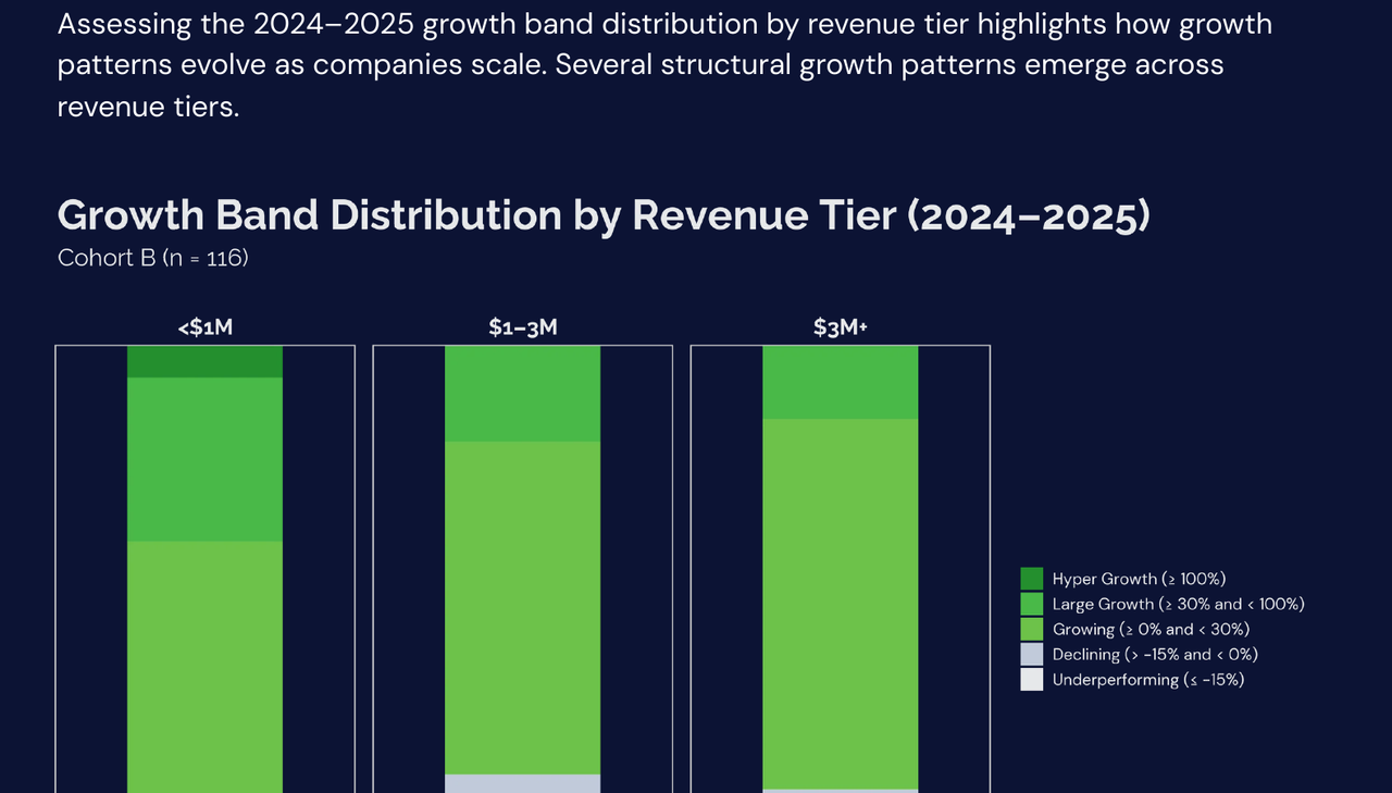
| Growth Band | <$1M (n=52) | $1–3M (n=41) | $3M+ (n=23) |
|---|---|---|---|
| Hyper Growth (≥ 100%) | 5.8% (3) | — | — |
| Large Growth (≥ 30% and < 100%) | 28.8% (15) | 17.1% (7) | 13.0% (3) |
| Growing (≥ 0% and < 30%) | 55.8% (29) | 58.5% (24) | 65.2% (15) |
| Declining (> -15% and < 0%) | 1.9% (1) | 19.5% (8) | 21.7% (5) |
| Underperforming (≤ -15%) | 7.7% (4) | 4.9% (2) | — |
Note: Hyper-growth outcomes were not observed in the $1–3M and $3M+ tier during the study period. Also, no underperforming companies were observed on the $3M+ tier
Small operators dominate the high-growth tail
Among companies below $1M, more than one-third achieve growth above 30%, and hyper-growth outcomes appear only within this tier. The smaller revenue base allows for rapid percentage expansion as operators scale routes, technicians, and marketing investment.
Mid-sized operators experience the sharpest growth compression
In the $1–3M segment, hyper-growth disappears and the share of companies achieving large growth declines by roughly half compared with the <$1M tier. At the same time, nearly one-fifth of operators report declining revenue, indicating that increasing organizational complexity begins to offset early-stage expansion momentum.
Larger operators shift toward steadier but less explosive growth
Companies above $3M cluster heavily within the moderate growth band (0–30%). While some contraction occurs as markets mature and year-over-year comparisons become more demanding, growth outcomes tend to be more stable and less volatile than those observed among smaller peers.
Overall, patterns in both the revenue growth distribution and growth band across revenue tiers signal a common scaling trajectory: rapid early expansion, a mid-market compression phase, and eventual stabilization as operational systems mature.
5.5 Regional Growth Context
Revenue Growth outcomes vary meaningfully across regions, reflecting differences in local market dynamics, operator maturity, and competitive intensity. While all regions exhibit broadly positive growth, dispersion across operators remains significant.
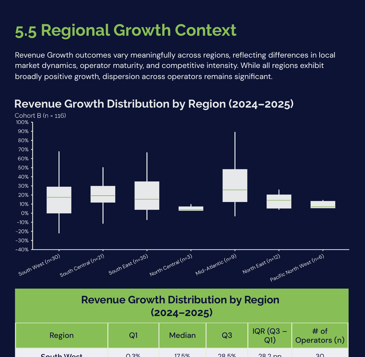
| Region | Q1 | Median | Q3 | IQR (Q3 – Q1) | # of Operators (n) |
|---|---|---|---|---|---|
| South West | 0.3% | 17.5% | 28.5% | 28.2 pp | 30 |
| South Central | 12.2% | 19.3% | 29.4% | 17.2 pp | 21 |
| South East | 4.2% | 15.3% | 34.3% | 30.1 pp | 35 |
| North Central | 3.3% | 3.7% | 6.8% | 3.5 pp | 3 |
| Mid-Atlantic | 12.8% | 25.6% | 47.8% | 35.0 pp | 9 |
| North East | 5.7% | 14.2% | 20% | 14.3 pp | 12 |
| Pacific North West | 6% | 7% | 12.9% | 6.90 pp | 6 |
Median growth ranges from 3.7% in North Central to 25.6% in the Mid-Atlantic, indicating that growth conditions vary across regional markets. However, variability within regions remains substantial, ranging from 3.5 pp to 35 pp, reinforcing that operator execution and local market positioning play a significant role in determining outcomes.
Regional Growth Band
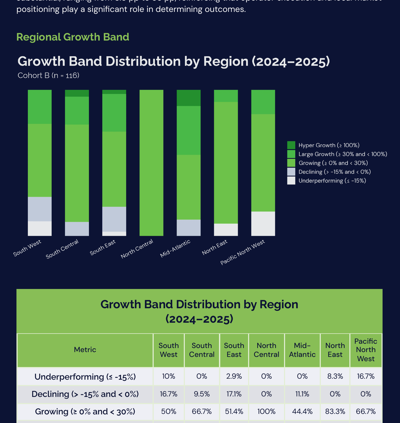
| Metric | South West | South Central | South East | North Central | Mid-Atlantic | North East | Pacific North West |
|---|---|---|---|---|---|---|---|
| Underperforming (≤ -15%) | 10% | 0% | 2.9% | 0% | 0% | 8.3% | 16.7% |
| Declining (> -15% and < 0%) | 16.7% | 9.5% | 17.1% | 0% | 11.1% | 0% | 0% |
| Growing (≥ 0% and < 30%) | 50% | 66.7% | 51.4% | 100% | 44.4% | 83.3% | 66.7% |
| Large Growth (≥ 30% and < 100%) | 23.3% | 19% | 25.7% | 0% | 33.3% | 8.3% | 16.7% |
| Hyper Growth (≥ 100%) | 0% | 4.8% | 2.9% | 0% | 11.1% | 0% | 0% |
Across most regions, the Growing or Moderate Growth Band (0–30%) captures most operators, indicating steady expansion across the industry, regardless of Region. However, the presence of both high-growth and declining operators in several regions highlights meaningful performance dispersion.
Regional Observations
Mid-Atlantic | Strongest Growth Momentum
The Mid-Atlantic region exhibits the strongest growth profile in the dataset, with median growth reaching 25.6% and the upper quartile approaching 47.8%. Over 44% of operators achieved growth above 30%, including 11.1% reaching hyper-growth levels. Notably, no operators in this region reported severe contraction.
South Central and South East | Balanced Expansion
South Central and South East demonstrate balanced growth distributions. Median growth reaches 19.3% and 15.3%, respectively, with strong representation in the moderate growth band. Large-growth outcomes are also common, with roughly 19–26% of operators exceeding 30% growth.
South West | Higher Dispersion
The South West shows greater variability in outcomes. While median growth remains solid at 17.5%, roughly 27% of operators experienced negative growth, alongside a meaningful share achieving strong expansion. This indicates a more polarized performance environment.
North East | Moderate but Stable
The North East demonstrates moderate but relatively stable growth, with median growth at 14.2% and most operators clustered in the moderate growth band.
Pacific North West | Slower Expansion
The Pacific North West shows slower growth dynamics, with median growth of 7.0%. Most operators fall within the moderate growth range, indicating steady but more measured expansion.
North Central | Limited Sample
The North Central region reports the lowest median growth at 3.7%, though the sample size is limited (n = 3). Results should therefore be interpreted cautiously.
Regional Data Considerations
Regional analysis is based on 116 operators with complete 2024–2025 revenue data. Participation varies significantly by region, with larger samples in the South East (n = 35) and South West (n = 30) providing more reliable signals.
Smaller samples particularly North Central (n = 3) and Pacific North West (n = 6) should be interpreted as directional rather than definitive.
Broadly, the regional analysis suggests that growth dispersion across operators is often greater than differences between regions themselves, indicating that operator execution, pricing strategy, and service mix likely play a larger role in growth outcomes than geography alone.
5.6 Chapter Summary: Growth is Non-Linear with Scale
Growth across pest control operators does not progress linearly with revenue size. Instead, the data suggests a three-stage scaling pattern:
- Small operators grow rapidly but with high variability.
- Mid-sized operators encounter structural friction as organizational complexity increases.
- Larger operators stabilize as operational systems, pricing discipline, and route density mature.
Scaling from <$1M to $3M+ therefore requires more than market demand. It typically requires operating redesign, including stronger technician management systems, clearer pricing discipline, route optimization, and more formalized sales infrastructure.
Operators that fail to adapt their operating structure during this transition often experience a prolonged mid-tier plateau, where growth slows despite continued market opportunity. The data indicates this inflection point is driven less by demand conditions and more by internal operational complexity.
Across both regional and revenue-tier views, the data shows that while geographic market conditions influence growth potential, structural factors, particularly scale, operating systems, and growth strategy, may play a more important role in shaping long-term performance outcomes.
tldr; Chapter 5 — Revenue Performance Trends (2023–2025)
Summary Points
- The industry is still growing, but growth is normalizing. Median Revenue Growth was 15.4% between 2024 and 2025. That is healthy. But the share of operators experiencing meaningful contraction increased from 1.7% in the prior period to 8.3%. Growth is still the norm, but it is becoming less uniform.
- 84% of operators grew. Non-negative growth was the rule, not the exception. But 17.3% of operators experienced some level of revenue decline, a reminder that this industry is not immune to execution risk, pricing pressure, or competitive intensity.
- Growth follows a three-stage pattern by revenue tier. Under $1M operators grow fastest but with the most variability (median 20.6%). The $1M to $3M range is the transition zone, where growth slows sharply to 9.9% as organizational complexity rises. Operators above $3M stabilize at 15.8% with tighter dispersion.
- The $1M to $3M tier is the hardest stage. This is not a performance problem. It is a structural one. Companies at this scale are building the management, staffing, and sales infrastructure required for the next phase. Growth often slows not because demand dried up, but because the operating model is being rebuilt.
- Regional differences are real but not deterministic. Median growth ranged from 3.7% in North Central to 25.6% in Mid-Atlantic. But within every region, the variation between operators was wider than the variation between regions. Where you operate matters less than how you operate.
- Growth consistency matters as much as growth rate. About 68% of operators in the three-year cohort showed positive revenue growth in both periods. Nearly one-third did not. Reliable recurring revenue through customer retention and route density is a stronger foundation than peak-year expansion.

Revenue Growth across the pest control industry has remained positive, though signs of moderation have emerged between 2024 and 2025. When growth begins to normalize, the relationship between expansion and profitability is increasingly determined by how effectively operators manage rising costs alongside revenue gains.
This chapter examines expense behavior across participating operators, focusing on multi-year cost structure trends, growth efficiency, and the cost drivers most closely linked to Margin performance.
Unless otherwise noted, analyses are based on Cohort B (n = 116) operators with full-year comparability between 2024 and 2025. Multi-year trend analysis references Cohort A (n = 60) operators with complete financial data from 2023–2025.
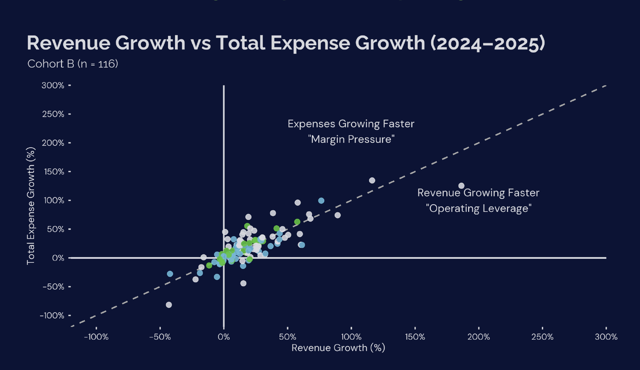
6.1 Revenue Growth vs Expense Growth (2024–2025)
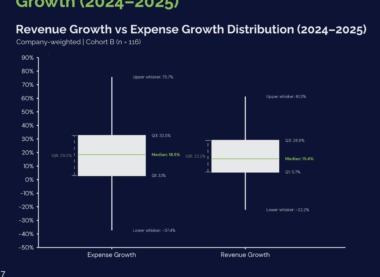
| Quartile | Expense Growth | Revenue Growth |
|---|---|---|
| Q1 (25th percentile) | 3.1% | 5.7% |
| Median | 18.5% | 15.4% |
| Q3 (75th percentile) | 32.5% | 28.9% |
| IQR (Q3–Q1) | 29.4 pp | 23.2 pp |
Common misread: Higher median values are not always better. For Expense Growth, lower values indicate greater efficiency, as slower cost expansion reflects stronger cost control.
While top-line growth appears healthy, with median revenue increasing by 15.4% from 2024 to 2025 and an interquartile range of 23.2 percentage points, the cost side of the equation presents a more nuanced and often overlooked story. Growth naturally brings higher costs, but not all cost expansion scales evenly with revenue. Beneath the surface, overall Expense Growth was both more dispersed and structurally higher, with the middle 50% of companies seeing expenses increase between 3.1% (Q1) and 32.5% (Q3), representing a wider spread of 29.4 percentage points. This indicates that cost expansion outpaced Revenue Growth for a meaningful portion of operators. At the same time, the spread of results suggests that efficient scaling remains achievable as some operators were able to control cost expansion despite similar growth conditions.
The gap between revenue and Expense Growth provides evidence that a meaningful portion of operators are scaling without maintaining cost alignment. This pattern shows that while revenue is increasing, many operators are spending more to get there, with costs growing faster than the business itself.
Operators should shift focus from growth alone to how costs are scaling alongside revenue. Start by identifying the largest areas of cost expansion and assessing whether these increases are intentional and aligned with business needs. If expenses are growing faster than revenue, resist adding new costs and focus on correcting the drivers of increase such as improving technician utilization before hiring, validating marketing efficiency before scaling spend, and tightening overhead as the business scales. The goal is not to slow down growth, but to ensure that cost expansion remains controlled and aligned as the business scales.
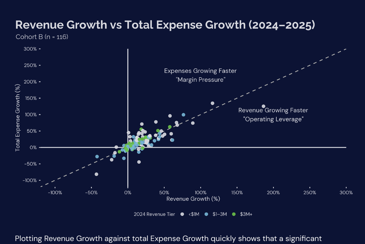
Plotting Revenue Growth against total Expense Growth quickly shows that a significant number of operators cluster close to the diagonal line, where costs rise with the same rate as revenue. However, equivalence between Revenue Growth and Expense Growth is not sufficient to create efficient gains or better Margins. Of the 116 operators analyzed, 56 experienced Expense Growth outpacing revenue, while 60 achieved Revenue Growth ahead of expenses, representing a near-even split between less efficient and more efficient growth outcomes.
Operators above the diagonal line, where Expense Growth exceeds Revenue Growth, are expanding their cost base faster than their top line, indicating rising cost intensity and Margin pressure.
Conversely, operators below the diagonal line demonstrate stronger operating leverage, with Revenue Growth outpacing expense expansion. These businesses were able to scale with relatively less incremental cost, creating operating leverage.
At a cohort level, this distribution highlights a key structural divide: growth efficiency varies widely across operators. Companies with similar Revenue Growth trajectories can operate very differently depending on how effectively costs scale alongside that growth.
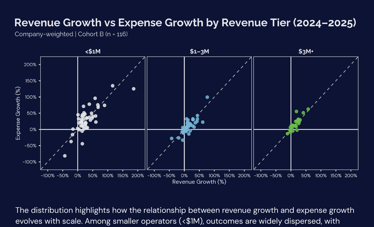
The distribution highlights how the relationship between revenue growth and expense growth evolves with scale. Among smaller operators (<$1M), outcomes are widely dispersed, with points spread across both sides of the diagonal. This indicates inconsistent cost control, where some operators successfully translate growth into operating leverage, while others experience expense growth that outpaces revenue, creating margin pressure. This variability reflects the challenges of scaling labor, absorbing overhead, and managing growth investment on a smaller scale.
As operators grow, this dispersion narrows. In the $1–3M tier, results begin to cluster more closely around the diagonal, suggesting improved alignment between revenue expansion and cost growth. By the time operators reach $3M+, the distribution tightens further, with most companies operating within a narrower range. This reflects greater cost discipline, more predictable scaling of labor, and stronger operating control as businesses mature.
Across all tiers, a consistent pattern emerges: many operators cluster near the diagonal, where revenue and expenses grow at similar rates. This indicates that growth alone does not inherently translate into margin expansion. Instead, the ability to maintain separation below the diagonal, where revenue growth exceeds expense growth, is what distinguishes more efficient operators.
The key takeaway is not whether operators achieved growth, but how efficiently that growth was delivered. Discipline on Cost-of-Service Expenses and Operating Expenses remain the primary determinant of whether revenue expansion translates into improved profitability.
6.2 Multi-Year Cost Structure Trend (2023–2025)
Multi-year trend analysis shows that the industry cost structure has remained broadly stable, although modest shifts across key expense categories have gradually influenced performance.
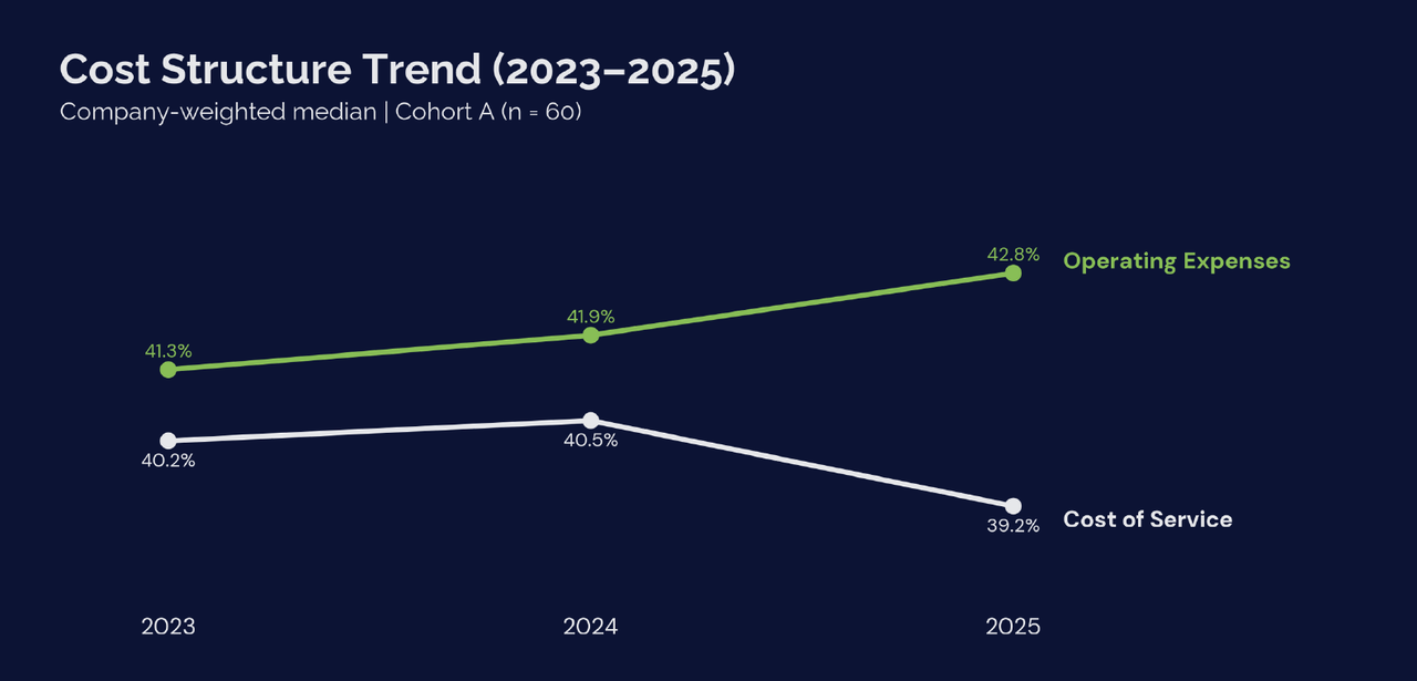
Across the 2023–2025 period, Cost of Service remains a significant component of the cost structure for pest control operators, though Operating Expenses represent a larger share at the median.
Cost of Service includes technician labor, service vehicles, materials, small equipment and chemicals, and other direct field costs associated with delivering service. Median COS increased from 40.2% in 2023 to 40.5% in 2024, before declining to 39.2% in 2025, indicating modest improvements in field-level cost efficiency in the most recent period.
On the other hand, Median Operating Expenses, which include indirect labor, sales and marketing, facility costs, and administrative overhead, increased from 41.3% in 2023 to 41.9% in 2024 and further to 42.8% in 2025. This trend indicates sustained upward pressure on overhead and support functions as companies scale, with that pressure becoming more pronounced in the most recent year.
| Metric | 2023 Median | 2024 Median | 2025 Median |
|---|---|---|---|
| Cost of Service % | 40.2% | 40.5% ▲ | 39.2% ▼ |
| Operating Expenses % | 41.3% | 41.9% ▲ | 42.8% ▲ |
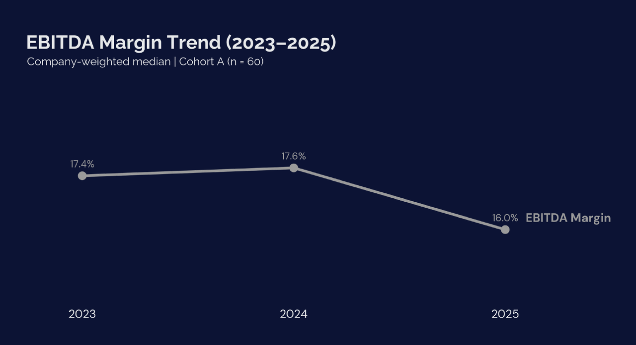
| EBITDA Margin % | 17.4% | 17.6% ▲ | 16.0% ▼ |
The time-series trend highlights an important shift in cost behavior across periods. From 2023 to 2024, median Cost of Service, OPEX, and EBITDA Margins all increased simultaneously, indicating that early-stage growth was supported by expanding cost structures without immediately eroding Margins. This can make underlying cost pressures less visible, allowing it to build as companies scale.
The pattern shifts from 2024 to 2025. Beneath the surface, continued cost expansion begins to outpace the moderating rate of revenue growth. As growth slows, the impact of rising costs becomes more visible, placing pressure on EBITDA margins, which show signs of compression in the most recent period.
These movements illustrate how shifts across cost layers interact. Even though direct service costs improved in 2025, this was more than offset by continued increases in Operating Expenses and slowing down of top-line growth, contributing to the compression of median EBITDA Margin from 17.6% in 2024 to 16.0% in 2025.
The data points to a clear signal: while operators have made progress managing direct service costs, rising overhead has become a more prominent driver of the overall cost structure. As businesses scale, maintaining discipline in operating expenses will be critical to sustaining performance.
The cost structure trend indicates that recent changes are increasingly driven by operating expenses rather than direct service costs. The analysis therefore focuses on the expense mix by component to identify the specific sources of pressure.
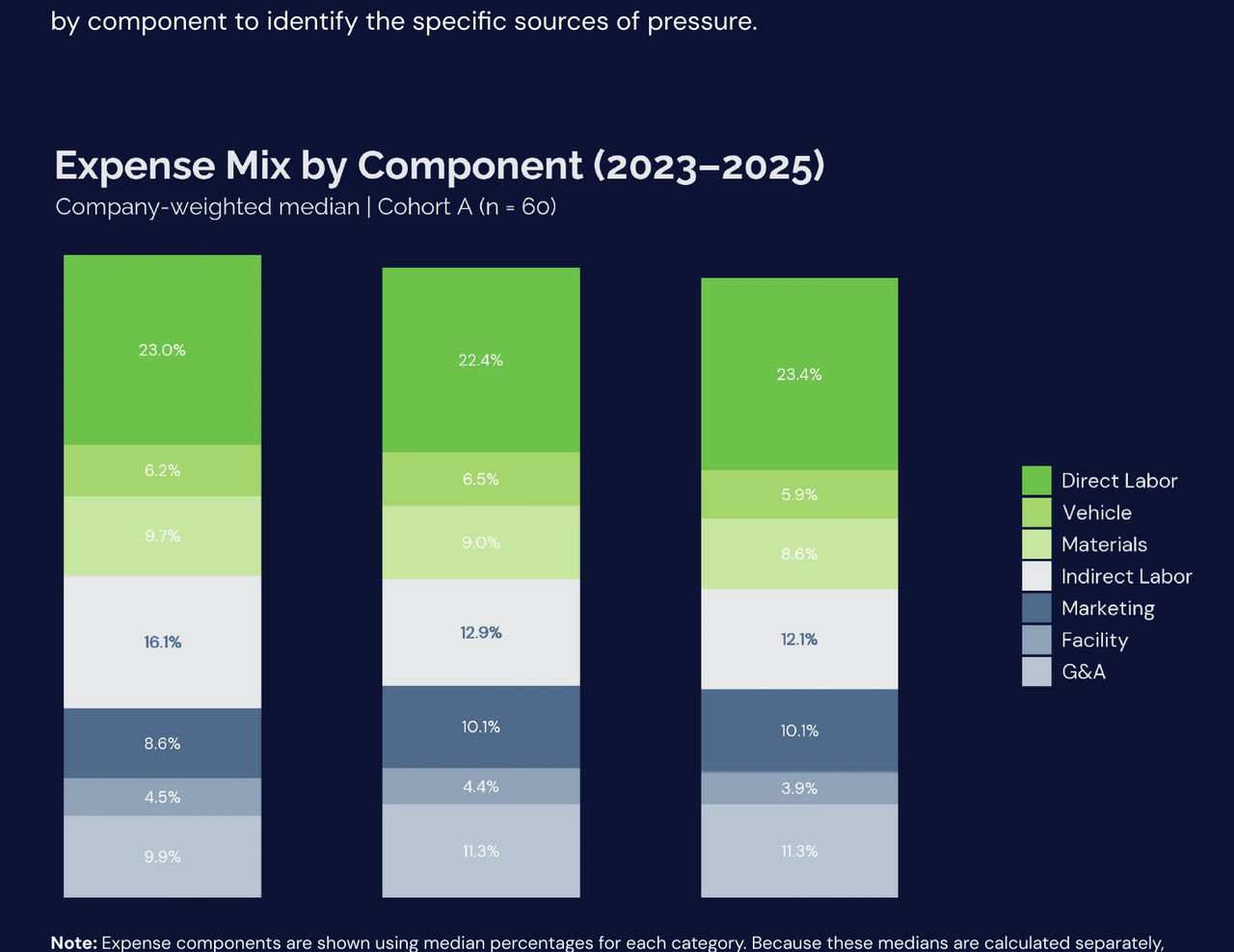
Note: Expense components are shown using median percentages for each category. Because these medians are calculated separately, the stacked totals are intended to show the relative mix of costs rather than to exactly add up to the overall COS, OPEX, or EBITDA Margin.
Breaking down expenses by component shows that the industry cost structure remains heavily concentrated in labor-related categories. Direct service labor continues to represent the largest single expense category across operators, highlighting the importance of continued efficiency which was seen earlier.
Marketing, facilities, and general and administrative costs account for smaller portions of the expense base but form the core overhead supporting operations and growth. Across the three-year period, the relative composition of these components remained broadly stable.
This consistency on the expense mix for the 3 periods indicates that much of the industry's cost structure is structural rather than cyclical. Personnel costs, both direct and indirect, remain the largest component of total expenses, meaning that even modest changes in labor productivity or staffing structure can have a meaningful impact on overall cost levels.
As a result, the focus shifts from broad cost reduction to disciplined cost scaling. Labor and overhead must grow in step with the business, maintaining technician productivity while ensuring that support functions, including management layers, administrative staff, and marketing infrastructure, remain aligned with operational needs.
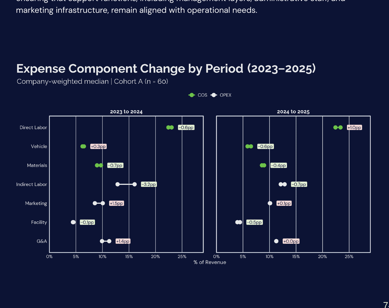
Year-over-year changes highlight where cost pressures have emerged. Between 2023–2024 and 2024–2025, several direct service cost categories stabilized or declined modestly. The main exception was direct labor, which increased by approximately one percentage point from 2024 to 2025.
In contrast, overhead categories, particularly marketing and G&A costs, showed more consistent upward movement across operators. Indirect labor, however, demonstrated the most noticeable improvement over the 2023–2025 period, suggesting that some operators have begun moderating the growth of support functions.
These observations shows that recent cost pressure reflects a combination of rising field labor costs and continued increase on growth investment as businesses scale. While several direct service costs stabilized or declined, increases in technician labor and ongoing investment in support functions continue to shape the overall cost structure.
Maintaining balance in cost structure will require operators to manage both sides of the equation, improving field productivity while ensuring that overhead growth remains aligned with operational needs.
Common Misreads:
- A stable expense mix does not mean costs are flat, absolute dollar value costs may still increase as the business grows.
- Lower COS does not necessarily indicate improved cost position if overhead expenses expand at the same time.
- Cost management is not about "cutting everything," but about identifying and addressing the largest and most impactful cost drivers.
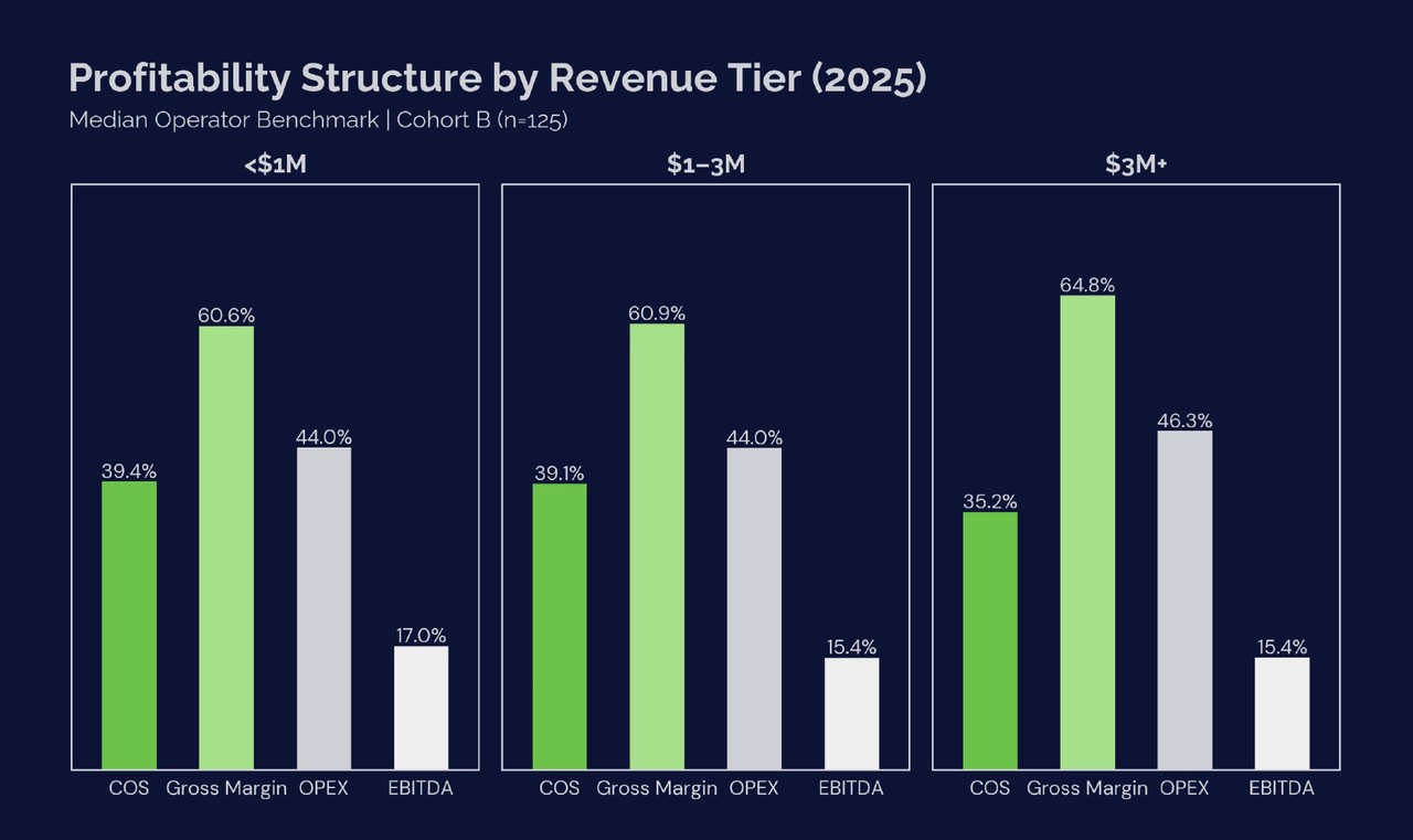
6.3 Cost Structure by Revenue Tier (2024–2025)
Cost structure varies meaningfully by company scale. Examining expense ratios and EBITDA Margin across revenue tiers highlights how operational complexity and scale influence the balance between field delivery costs and overhead.
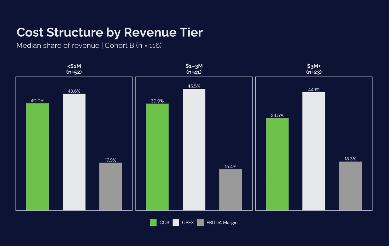
| 2024 Revenue Tier | COS | OPEX | Margin |
|---|---|---|---|
| <$1M | 40.0% | 43.6% | 17.9% |
| $1–3M | 39.9% | 45.5% | 15.4% |
| $3M+ | 34.5% | 44.1% | 18.3% |
Several structural patterns emerge across the revenue groups. Larger operators ($3M+) tend to operate with lower Cost of Service ratios, reflecting stronger route density, improved technician utilization, and more developed operational systems. However, these efficiencies are partially offset by the higher overhead required to support larger organizational structures.
Notably, the $1–3M tier exhibits the lowest median EBITDA Margin, indicating that companies in this range often experience a transitional phase where organizational complexity begins to increase faster than operational efficiency.
These patterns illustrate how cost structures evolve as companies scale. Operators generating less than $1M in revenue typically operate with lean administrative structures and rely more heavily on owner-operators or small technician teams. As a result, a larger share of revenue is often allocated to direct service delivery costs.
Companies in the $1–3M tier often begin adding operational infrastructure, including dispatch functions, office staff, and expanded technician teams. These additions increase operating overhead but also support greater service capacity and growth potential.
At the $3M+ level, organizations typically introduce more formal management layers, sales infrastructure, and administrative support. While these additions increase overhead, larger operators often benefit from improved route density, stronger pricing discipline, and greater operating leverage.
These dynamics point to a clear operational implication: as businesses scale, the challenge is not simply adding capacity but ensuring that each layer of overhead is introduced in line with measurable gains in productivity. In practice, this means actively managing technician utilization, monitoring revenue per employee, and aligning support functions to field output, rather than allowing overhead to expand ahead of operational needs.
6.4 Expense Scaling Patterns (2024–2025)
Despite strong Revenue Growth across the cohort, bottom-line profitability outcomes were mixed. Median EBITDA Margin increased by only +0.24 percentage points, indicating that revenue expansion and cost growth moved largely in tandem for a typical operator. In other words, the industry did not experience a meaningful marginal improvement in profitability during the period.
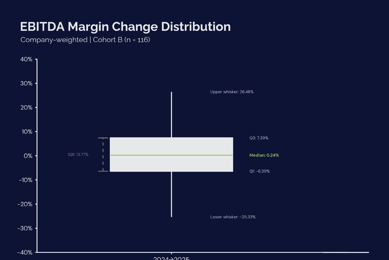
| Metric | Value |
|---|---|
| Q1 (25th percentile) | -6.39% |
| Median | 0.24% |
| Q3 (75th percentile) | 7.39% |
| IQR (Q3–Q1) | 13.77 pp |
Although the overall cohort showed limited change in median EBITDA Margin between 2024 and 2025, outcomes varied meaningfully across operators. While the median result was essentially flat at 0.24%, the distribution shows that some companies expanded Margins significantly while others experienced notable contraction. This indicates that Revenue Growth alone did not determine profitability; the more important factor was how effectively costs scaled alongside that growth.
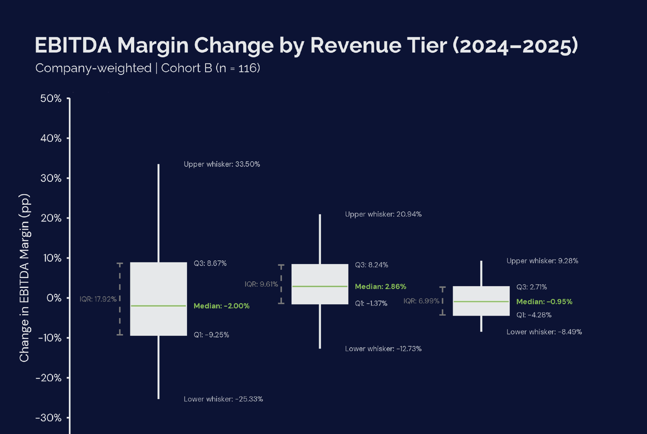
| 2024 Revenue Tier | Q1 | Median | Q3 | IQR |
|---|---|---|---|---|
| <$1M | -9.25% | -2.00% | 8.67% | 17.92 pp |
| $1–3M | -1.37% | 2.86% | 8.24% | 9.61 pp |
| $3M+ | -4.28% | -0.95% | 2.71% | 6.99 pp |
When segmented by revenue tier, EBITDA margins differ clearly across tiers. Smaller operators below $1M exhibited the widest dispersion in outcomes, with some companies achieving significant expansion while others experienced meaningful declines. This volatility reflects the scale sensitivity of smaller businesses. Notably, despite recording the strongest median Revenue Growth, this tier experienced median EBITDA Margin compression, indicating that costs scaled faster than revenue for the typical operator on this tier.
Operators in the $1–3M tier demonstrated the strongest median Margin improvement and the most balanced overall outcome. Margin changes in this segment clustered more tightly around the median. While larger operators often benefit from stronger field productivity and route density, operators in this range were better able to absorb cost pressures while preserving operating efficiency. This appears to be the point where route density, technician utilization, and overhead absorption begin to stabilize operating economics more effectively.
Among operators above $3M, Margin outcomes were comparatively stable but slightly weaker at the median. While larger operators often benefit from stronger field productivity and route density, these benefits can be partially offset by overhead expansion. As scale grows, cost optimization, the expansion of administrative infrastructure and management layers can introduce additional overhead that partially offsets operating leverage.
Across the three tiers, variability decreases as revenue scale increases. The interquartile range narrows at higher revenue levels, reinforcing earlier observations that larger operators tend to exhibit more consistent, though less volatile, performance.
Overall, the data reinforces a key benchmark insight: scale alone does not guarantee Margin expansion. Profitability depends on how effectively operators manage both field productivity and overhead growth as the business expands.
Component-Level Cost Pressure (2024–2025)
Examining component-level cost movements helps explain why Margin outcomes diverged across the cohort. At the overall benchmark level, median cost share of revenue increased modestly in labor-related and administrative categories, while Materials, Facility, Vehicle, and Sales & Marketing declined slightly as a percentage of revenue. This indicates that recent Margin pressure was driven less by direct service inputs and more by labor and overhead expansion.
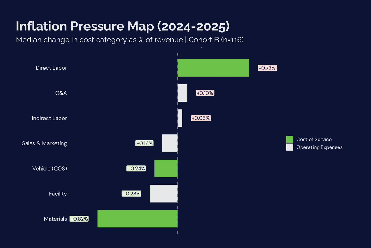
| Cost Driver | 2024 Median (% Rev) | 2025 Median (% Rev) | Change (pp) |
|---|---|---|---|
| Direct Labor | 22.00% | 22.73% | ▲ 0.73 |
| G&A | 11.40% | 11.50% | ▲ 0.10 |
| Indirect Labor | 12.70% | 12.75% | ▲ 0.05 |
| Sales & Marketing | 11.40% | 11.20% | ▼ 0.16 |
| Vehicle (COS) | 5.99% | 5.76% | ▼ 0.24 |
| Facility | 4.05% | 3.77% | ▼ 0.28 |
| Materials | 9.24% | 8.42% | ▼ 0.82 |
Viewed through a benchmarking lens, the Inflation Pressure Map tells a more precise story. Cost pressure was not evenly distributed across categories. The largest increase occurred in Direct Labor, while G&A and Indirect Labor also edged upward. In contrast, Materials, Facility, Vehicle, and Sales & Marketing all declined modestly as a share of revenue, indicating that some operators improved efficiency in procurement, facility utilization, fleet leverage, or customer acquisition spend.
These results indicate that Margin pressure during the period was influenced more by labor and administrative expansion than by direct input inflation alone.
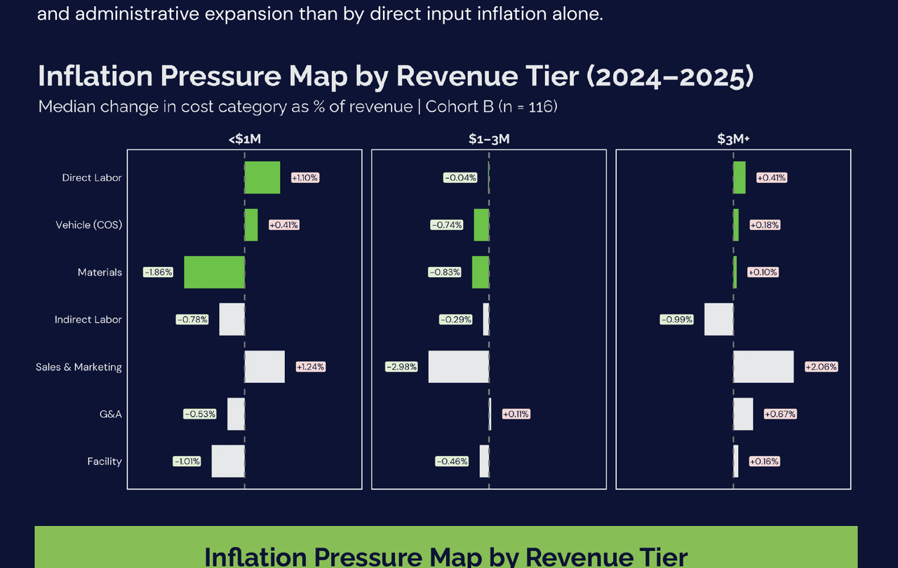
| 2024 Revenue Tier | Cost Driver | Category | 2024 Median (% Rev) | 2025 Median (% Rev) | Change (pp) |
|---|---|---|---|---|---|
| <$1M | Direct Labor | COS | 21.99% | 23.09% | ▲ 1.10 |
| Vehicle (COS) | COS | 6.03% | 6.44% | ▲ 0.41 | |
| Materials | COS | 11.65% | 9.79% | ▼ 1.86 | |
| Indirect Labor | OPEX | 10.68% | 9.90% | ▼ 0.78 | |
| Sales & Marketing | OPEX | 8.82% | 10.06% | ▲ 1.24 | |
| G&A | OPEX | 12.47% | 11.94% | ▼ 0.53 | |
| Facility | OPEX | 4.71% | 3.70% | ▼ 1.01 | |
| $1–3M | Direct Labor | COS | 22.82% | 22.78% | ▼ 0.04 |
| Vehicle (COS) | COS | 6.51% | 5.76% | ▼ 0.74 | |
| Materials | COS | 9.17% | 8.34% | ▼ 0.83 | |
| Indirect Labor | OPEX | 15.75% | 15.46% | ▼ 0.29 | |
| Sales & Marketing | OPEX | 13.11% | 10.13% | ▼ 2.98 | |
| G&A | OPEX | 11.42% | 11.53% | ▲ 0.11 | |
| Facility | OPEX | 4.45% | 3.98% | ▼ 0.46 | |
| $3M+ | Direct Labor | COS | 21.24% | 21.65% | ▲ 0.41 |
| Vehicle (COS) | COS | 5.07% | 5.25% | ▲ 0.18 | |
| Materials | COS | 6.49% | 6.60% | ▲ 0.10 | |
| Indirect Labor | OPEX | 11.58% | 10.59% | ▼ 0.99 | |
| Sales & Marketing | OPEX | 14.28% | 16.34% | ▲ 2.06 | |
| G&A | OPEX | 9.21% | 9.88% | ▲ 0.67 | |
| Facility | OPEX | 3.14% | 3.31% | ▲ 0.16 |
When viewed by revenue tier, cost pressure reveals distinct scaling dynamics across operator sizes. Sub-$1M operators experienced the clearest labor pressure. Direct Labor and Sales & Marketing both increased as a share of revenue, while Vehicle costs also rose modestly. At the same time, these operators improved in Materials, Facility, Indirect Labor, and G&A. This indicates that smaller businesses may have faced greater wage sensitivity or lower technician productivity during the period, even while maintaining relatively lean overhead structures elsewhere.
Operators in the $1–3M range showed the broadest signs of efficiency improvement. Sales & Marketing, Materials, Vehicle, Facility, and Indirect Labor all declined as a share of revenue, while Direct Labor remained effectively flat. This pattern indicates that many mid-sized operators were able to improve cost absorption and operating discipline as revenue scaled, with only modest pressure emerging in G&A.
Among operators above $3M, cost pressure shifted more clearly toward overhead and growth infrastructure. Sales & Marketing rose sharply, while G&A, Facility, and Vehicle also increased. Direct Labor moved higher as well, though less dramatically. These movements indicate that larger operators faced Margin pressure from the cost of supporting a more complex organization and growth engine.
The data and analysis show that Margin pressure was not concentrated in a single category across much of the industry. Instead, it manifested differently by company size. Smaller operators appear more exposed to labor volatility, mid-sized operators showed the strongest evidence of cost absorption, and larger operators increasingly faced the structural cost expansion associated with broader administrative and commercial infrastructure.
For operators, regardless of scale, the implication is clear: improving Margins is not simply a function of growing revenue, but of managing the right costs at the right stage of scale. Sustained profitability requires delicate balancing of technician productivity, customer acquisition efficiency and careful control of administrative overhead as the organization grows.
6.5 Regional Cost Differences (2024–2025)
Regional operating conditions can influence both cost structure and profitability through differences in labor markets, facility costs, competition intensity and customer acquisition dynamics. To evaluate whether these factors materially affect benchmark performance, this section compares Cost of Service, Operating Expenses, and EBITDA Margin across regions within the 2024–2025 benchmark cohort.
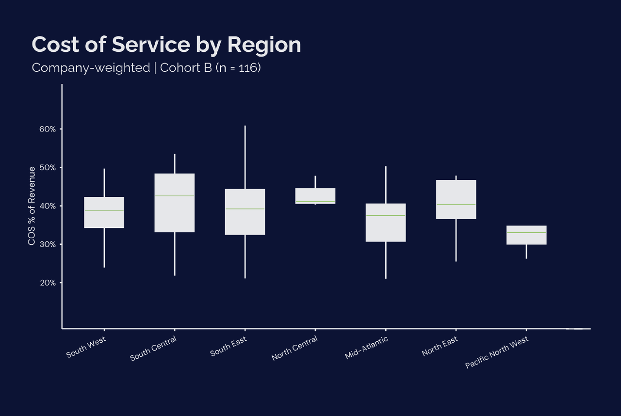
| Region | Q1 | Median | Q3 | IQR | n |
|---|---|---|---|---|---|
| South West | 34.4% | 38.9% | 42.1% | 7.7 pp | 30 |
| South Central | 33.3% | 42.6% | 48.2% | 14.9 pp | 21 |
| South East | 31.4% | 39.0% | 43.9% | 12.5 pp | 35 |
| North Central | 40.7% | 41.1% | 44.5% | 3.8 pp | 3 |
| Mid-Atlantic | 30.9% | 37.4% | 40.4% | 9.5 pp | 9 |
| North East | 36.7% | 40.4% | 46.5% | 9.8 pp | 12 |
| Pacific North West | 30.1% | 33.0% | 34.7% | 4.6 pp | 6 |
Direct service costs showed overall consistency with pockets of variation across regions, reflecting differences in technician labor costs, route density, and service delivery efficiency. While median Cost of Service ranged from 33.0% to 42.6% of revenue, IQRs of 4.6 to 14.9 percentage points indicate that outcomes remained relatively stable within regions.
Operators in South Central recorded the highest median COS at 42.6%, followed by North Central (41.1%) and North East (40.4%), indicating relatively higher direct service costs in those markets. By contrast, Pacific North West operators recorded the lowest median COS at 33.0%, indicating comparatively stronger field cost efficiency.
Other regions clustered more tightly around the middle of the distribution, including South East (39.0%), South West (38.9%), and Mid-Atlantic (37.4%), indicating broadly similar service delivery economics across much of the cohort.
Overall, while regional labor conditions and route density influence technician productivity, the relatively contained COS range reinforces the underlying consistency of core field service economics across the pest control industry.

| Region | Q1 | Median | Q3 | IQR | n |
|---|---|---|---|---|---|
| South West | 38.2% | 44.5% | 60.2% | 22.0 pp | 30 |
| South Central | 34.2% | 45.7% | 48.5% | 14.3 pp | 21 |
| South East | 31.0% | 39.4% | 49.1% | 18.1 pp | 35 |
| North Central | 42.0% | 42.6% | 43.3% | 1.3 pp | 3 |
| Mid-Atlantic | 42.2% | 44.9% | 51.9% | 9.7 pp | 9 |
| North East | 44.1% | 46.9% | 53.1% | 9.0 pp | 12 |
| Pacific North West | 37.0% | 45.4% | 56.2% | 19.2 pp | 6 |
Overhead costs displayed slightly greater variation than direct service costs across regions. Median Operating Expenses ranged from 39.4% to 46.9% of revenue.
Operators in the North East recorded the highest median overhead levels at 46.9%, followed by South Central (45.7%), Pacific North West (45.4%), and Mid-Atlantic (44.9%). These higher overhead ratios may reflect differences in administrative staffing structures, facility costs, and growth-related spending across markets.
By comparison, South East operators maintained the leanest overhead structure at 39.4%, indicating relatively lighter administrative cost burdens. South West (44.5%) and North Central (42.6%) fell closer to the middle of the distribution.
These results hint that while direct service economics remain relatively stable across markets, overhead structures can vary more noticeably depending on organizational scale, management layers, and regional operating practices.
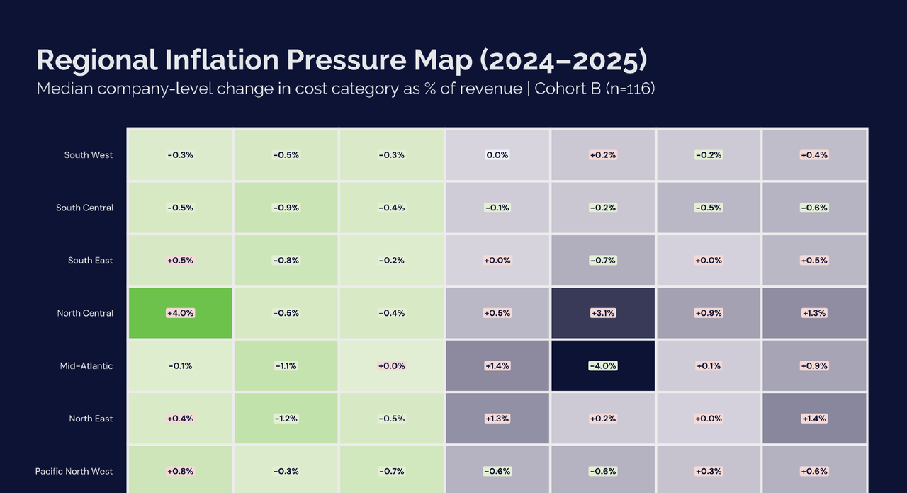
To better understand the drivers behind regional profitability differences, cost inflation was examined by category across each geographic market. The table above shows the median change in cost share of revenue between 2024 and 2025 across the Growth Cohort (n = 116).
Across most regions, cost pressures were relatively balanced. Modest increases in administrative expenses and technician labor were partially offset by improvements in materials and customer acquisition efficiency.
Materials costs declined as a percentage of revenue in nearly every region, indicating that pricing adjustments, service mix changes, or procurement efficiencies helped offset chemical and product cost inflation.
Labor dynamics varied more noticeably across markets. The Pacific North West and South East recorded the largest increases in Direct Labor share, rising approximately 0.8% and 0.5% of revenue, respectively. These increases likely reflect wage pressure and technician capacity constraints in tighter labor markets.
Administrative expenses also rose in several regions. G&A increased by 1.4% in the North East, 0.9% in the Mid-Atlantic, and 0.6% in the Pacific North West, reflecting continued investment in management infrastructure and administrative support as operators scale operations.
The North Central region stands out as a clear outlier. Direct Labor increased by roughly 4.0% of revenue, while Sales & Marketing rose 3.1% and G&A increased 1.3%. This simultaneous expansion across multiple cost categories corresponds with the sharp Margin compression observed in the regional Margin analysis. However, the regional sample size remains small (n = 3), meaning results are more sensitive to individual company performance.
Conversely, several regions demonstrated improvements in acquisition efficiency. Sales & Marketing declined by 4.0% of revenue in the Mid-Atlantic, 0.7% in the South East, and 0.6% in the Pacific North West, indicating that stronger recurring revenue programs and improved customer retention may have reduced reliance on new customer acquisition spending.
The regional inflation analysis reinforces a broader conclusion of this benchmark study: cost pressure within the pest control industry rarely originates from a single category. Instead, Margin outcomes typically reflect the combined influence of labor dynamics, overhead expansion, and acquisition efficiency within each operator's local market environment.
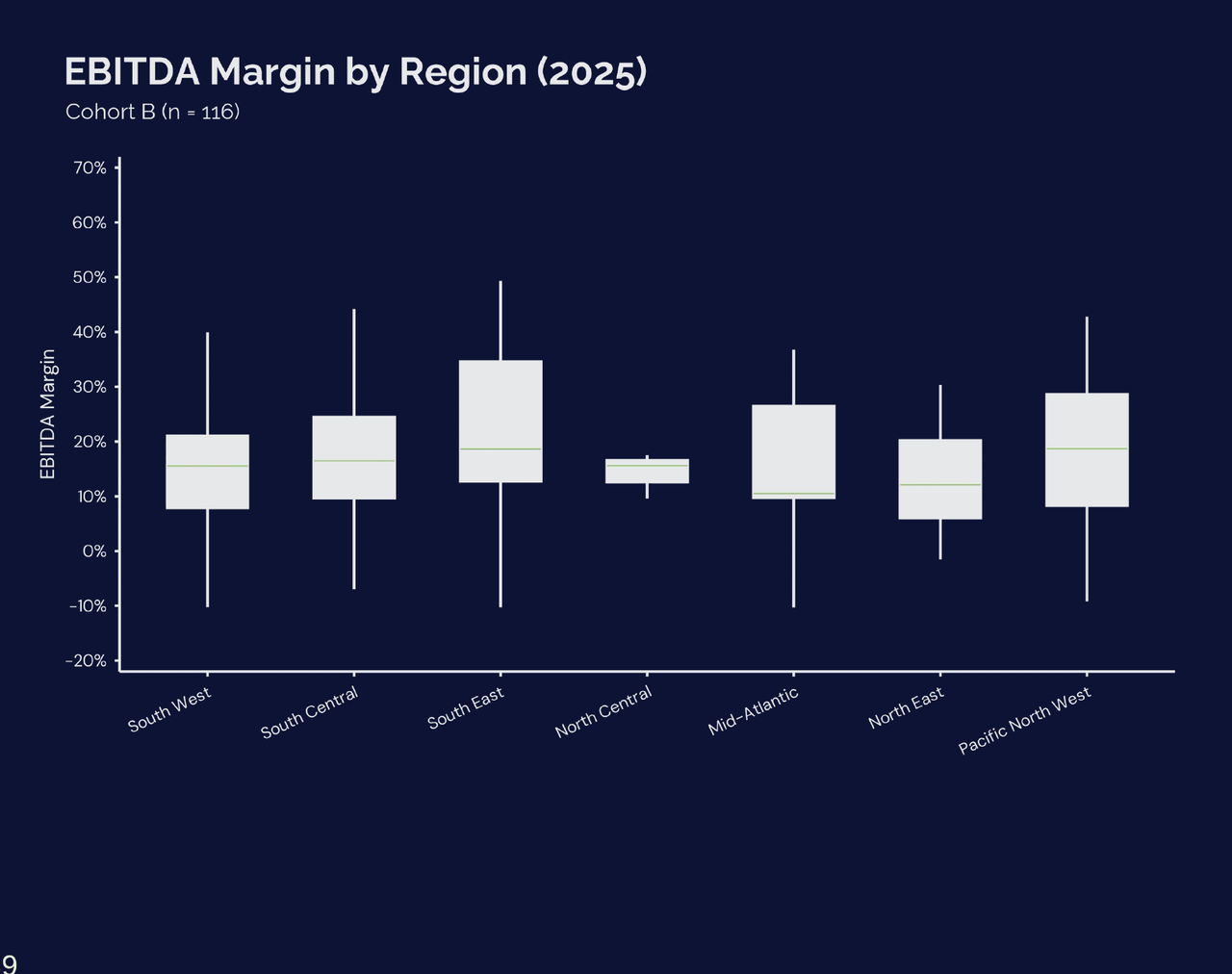
| Region | Q1 | Median | Q3 | IQR | n |
|---|---|---|---|---|---|
| South West | 3.6% | 15.2% | 20.5% | 16.9 pp | 30 |
| South Central | 9.6% | 16.5% | 24.4% | 14.8 pp | 21 |
| South East | 12.5% | 18.6% | 34.8% | 22.3 pp | 35 |
| North Central | 12.6% | 15.6% | 16.6% | 4.0 pp | 3 |
| Mid-Atlantic | 9.7% | 10.5% | 26.5% | 16.8 pp | 9 |
| North East | 4.0% | 10.3% | 20.1% | 16.1 pp | 12 |
| Pacific North West | 8.3% | 18.7% | 28.6% | 20.3 pp | 6 |
Despite differences in both direct and overhead costs, EBITDA Margins remained relatively consistent across most regions. Median EBITDA Margins ranged from 10.3% to 18.7%, indicating broadly comparable profitability levels across geographic markets.
Operators in the Pacific North West (18.7%) and South East (18.6%) recorded the highest median EBITDA Margins in the benchmark cohort. South Central (16.5%), North Central (15.6%), and South West (15.2%) followed closely.
Meanwhile, Mid-Atlantic (10.5%) and North East (10.3%) recorded the lowest median Margins, reflecting somewhat tighter operating economics across these markets.
However, the relatively narrow spread in median Margins indicates that operators frequently adjust pricing, service mix, and cost management practices to maintain broadly comparable profitability levels despite regional cost differences.
| Region | Q1 | Median | Q3 | IQR | n |
|---|---|---|---|---|---|
| South West | -5.9% | 0.0% | 5.3% | 11.2 pp | 30 |
| South Central | -0.3% | 4.0% | 9.1% | 9.4 pp | 21 |
| South East | -5.0% | 0.2% | 9.6% | 14.6 pp | 35 |
| North Central | -15.7% | -11.1% | -9.9% | 5.8 pp | 3 |
| Mid-Atlantic | 0.0% | 3.9% | 8.0% | 8.0 pp | 9 |
| North East | -7.4% | -3.1% | 0.0% | 7.4 pp | 12 |
| Pacific North West | -13.2% | 1.5% | 7.8% | 21.0 pp | 6 |
Changes in EBITDA Margins between 2024 and 2025 reveal additional variation across regional markets. While the overall benchmark cohort exhibited relatively flat changes on profitability Margins during the period, regional outcomes differed depending on how effectively operators managed Revenue Growth relative to cost expansion.
Operators in South Central recorded the strongest median Margin improvement (+4.0 percentage points), followed closely by Mid-Atlantic (+3.9 points). These improvements suggest that Revenue Growth in these markets outpaced cost increases during the period.
Margin performance was largely stable in South East (+0.2 points) and South West (approximately flat), indicating that Revenue Growth was largely offset by parallel increases in Operating Expenses.
Some regions experienced Margin contraction. North East operators saw median Margin decline of approximately –3.1 percentage points, while North Central recorded the largest contraction (–11.1 points). However, the small sample size in North Central makes these results more sensitive to individual company performance.
Overall, the regional Margin analysis reinforces a broader conclusion observed throughout this study: across much of the industry, Revenue Growth during the period was accompanied by corresponding cost expansion, resulting in relatively limited Margin improvement at the aggregate level. The data also shows that while local operating conditions influence cost structure and Margin variability, the core economics of pest control operations remain broadly consistent across markets. Differences in profitability appear to be driven more by operator execution and cost discipline than by structural geographic advantage alone.
6.6 Chapter Summary: How Cost Structure Shapes Profitability
Revenue Growth across the benchmark cohort remained strong during the period analyzed, reinforcing the continued expansion of the pest control industry. However, this chapter shows that growth alone does not automatically translate into profitability. The more critical factor is how effectively operators manage the cost structure that supports that growth, ensuring expenses do not scale at the same rate as, or faster than, revenue.
Across the cohort, Revenue Growth and Expense Growth generally moved in tandem. As a result, median EBITDA Margin change was basically flat (+0.24%) between 2024 and 2025. While some operators achieved meaningful operating leverage, where revenue expanded faster than cost, others experienced Margin compression as expenses grew at a similar or faster pace than revenue.
Multi-year trend analysis indicates that the overall industry cost structure has remained relatively stable in composition. Operating Expenses continue to represent the largest portion of the cost structure. At the same time, improvements in Cost-of-Service efficiency were partially offset by rising overhead expenses, especially within administrative and support functions. As companies scale, the operational challenge gradually shifts from managing field-level efficiency to maintaining discipline in the growth of organizational infrastructure.
Segmented revenue analysis further shows that cost dynamics vary by company size. Smaller operators exhibit greater volatility in Margin outcomes, reflecting higher sensitivity to labor productivity, staffing changes, and overhead absorption. Mid-sized operators often demonstrate the strongest cost absorption as revenue scales, while larger operators face increasing pressure from the administrative complexity and commercial infrastructure required to support larger organizations.
Regional comparisons suggest that while labor markets, pricing environments, and operating conditions differ geographically, the core economics of pest control operations remain broadly consistent across markets. Differences in profitability appear to be driven less by geography and more by execution, particularly pricing discipline, technician productivity, and overhead management.
The findings reinforce a central benchmark insight: sustainable profitability in pest control is not simply a function of growth, but of disciplined scaling. Operators who successfully convert revenue expansion into operating leverage tend to maintain technician productivity, manage overhead expansion carefully, and ensure that cost growth remains aligned with revenue productivity. A key takeaway of this chapter is that the industry continues to grow, but the operators who benefit most are those whose cost structures scale more slowly than their revenue.
tldr; Chapter 6 — Expense Patterns and Cost Drivers (2023–2025)
Summary Points
- Revenue and expenses are growing at the same rate for most operators. When you plot revenue growth against expense growth across the cohort, most operators cluster near the diagonal line. That means growth is not creating leverage. Costs are expanding in lockstep with the top line, and margins are not moving.
- Median EBITDA Margin barely changed. Between 2024 and 2025, the typical operator improved EBITDA Margin by just 0.24 percentage points. Revenue grew 15.4%. The money came in. And most of it went straight back out.
- Direct service costs improved slightly. Overhead got heavier. Median Cost of Service declined modestly to 39.2% in 2025. But median Operating Expenses climbed to 42.8%, up from 41.3% in 2023. The gains at the field level are being absorbed by administrative and support cost growth.
- Labor is the largest single cost at every tier. Direct technician labor, indirect staffing, and people-related costs combined represent the dominant share of the cost structure. Even small inefficiencies in scheduling, routing, or staffing levels compound quickly into margin pressure.
- Cost pressure looks different at each scale. Under $1M operators felt the most pressure in direct labor and marketing. The $1M to $3M tier showed the most efficiency improvement across nearly every category. Operators above $3M saw the sharpest rise in overhead and growth infrastructure costs.
- A stable expense mix is not the same as flat costs. The proportional composition of cost categories has stayed roughly consistent over three years. But as revenue grows, every percentage point represents more dollars. Discipline is not about cutting costs. It is about making sure each cost category earns its place.

11.1 Key Findings from the Benchmark
This benchmark study examined financial performance across 125 pest control operators, with 116 companies forming the comparable cohort for year-over-year growth analysis. The findings reveal several consistent structural patterns that characterize the economics of modern pest control businesses.
Across the cohort, median Revenue Growth between 2024 and 2025 was 15.4%, with the 50% of operators growing between 5.7% and 28.9%. This range reflects both strong expansion among many operators and meaningful variability in growth trajectories across the industry.
Profitability outcomes were more dispersed. Median EBITDA Margins reached 15.6% but ranged from 6.7% at the 25th percentile to 24.4% at the 75th percentile, highlighting the importance of operational efficiency and cost discipline in determining final profitability outcomes.
Cost structure benchmarks remained relatively consistent across the cohort. Median Gross Margins were approximately 61%, while total people costs consumed roughly 37% of revenue. Sales & Marketing spending averaged 11.2% of revenue, while Operating Expenses represented 43.9% of revenue at the median.
Taken together, these benchmarks confirm a central theme observed throughout the study: while Revenue Growth remains strong across the industry, profitability outcomes depend heavily on how effectively operators manage labor productivity, marketing investment, and overhead expansion as they scale.
11.2 Industry Planning Signals for 2026
Several shifts observed in the 2024–2025 data provide important context for operators planning their 2026 budgets.
- Growth remains healthy but uneven across the cohort Smaller operators continue to grow the fastest, with sub-$1M companies achieving median growth of 20.6%, compared with 9.9% for $1–3M operators and 15.8% for $3M+. At the same time, growth dispersion remains wide, reinforcing that outcomes vary significantly by operator execution.
- Profitability outcomes reflect modest Margin improvement and scale effects Gross Margin improvements appear modest but consistent among larger operators, indicating stronger Cost of Service efficiency as scale increases. However, these gains are not uniform across the cohort and are often partially offset by expanding Operating Expenses, resulting in more limited improvement in overall profitability.
- Cost structure remains labor-driven, with efficiency determining outcomes Labor continues to represent the largest cost lever across all tiers, making technician productivity and staffing efficiency critical to Margin performance. Marketing investment remains an important growth driver, but operators that manage acquisition efficiency more effectively tend to achieve stronger profitability outcomes.
These trends suggest that the most successful operators entering 2026 will be those that sustain growth while maintaining discipline in labor productivity, marketing efficiency, and overhead expansion.
11.3 Budget Guardrails by Revenue Tier
The following benchmarks provide practical budgeting reference points for operators planning the upcoming year.
| Metric | Q1 | Median | Q3 |
|---|---|---|---|
| Revenue Growth | 12.3% | 20.6% | 39.5% |
| Gross Margin | 54.5% | 60.6% | 66.2% |
| EBITDA Margin | 4.5% | 17.0% | 24.1% |
| Direct Labor | 16.6% | 22.6% | 26.9% |
| Direct Vehicle/Fleet | 4.48% | 6.49% | 8.44% |
| Materials / Chemicals | 7.5% | 10.2% | 13.5% |
| Marketing | 4.0% | 9.5% | 17.9% |
| Indirect People | 2.5% | 9.3% | 23.0% |
| Facility | 2.1% | 4.1% | 6.6% |
| G&A | 11.3% | 14.0% | 18.9% |
Smaller operators tend to grow faster but often face more variability in operating performance. Maintaining discipline around labor efficiency and marketing investment is particularly important at this stage of growth.
| Metric | Q1 | Median | Q3 |
|---|---|---|---|
| Revenue Growth | 3.4% | 9.9% | 27.5% |
| Gross Margin | 54.6% | 60.9% | 66.3% |
| EBITDA Margin | 6.8% | 15.4% | 24.5% |
| Direct Labor | 18.5% | 23.3% | 28.3% |
| Direct Vehicle/Fleet | 3.97% | 5.53% | 7.36% |
| Materials / Chemicals | 6.0% | 8.3% | 11.0% |
| Marketing | 7.4% | 13.5% | 21.0% |
| Indirect People | 10.9% | 14.7% | 19.3% |
| Facility | 2.7% | 3.8% | 5.1% |
| G&A | 9.1% | 10.9% | 14.6% |
Operators in this range typically experience increasing route density and operational stability but also begin to absorb more overhead as the business scales.
| Metric | Q1 | Median | Q3 |
|---|---|---|---|
| Revenue Growth | 2.9% | 15.8% | 24.4% |
| Gross Margin | 59.3% | 64.8% | 71.0% |
| EBITDA Margin | 7.8% | 15.4% | 29.4% |
| Direct Labor | 17.6% | 21.1% | 27.0% |
| Direct Vehicle/Fleet | 4.24% | 5.18% | 6.12% |
| Materials / Chemicals | 5.2% | 6.9% | 9.4% |
| Marketing | 10.2% | 15.5% | 26.9% |
| Indirect People | 9.6% | 12.1% | 15.6% |
| Facility | 2.7% | 3.3% | 4.2% |
| G&A | 8.4% | 10.5% | 13.1% |
Larger operators tend to demonstrate slightly stronger service-level Margins, although profitability ultimately depends on how effectively overhead and administrative complexity are managed.
11.4 Metrics Operators Should Monitor Monthly
To avoid gradual Margin erosion, operators should monitor several key metrics throughout the year.
The most important indicators include:
Revenue Growth
Tracking growth relative to plan ensures that fixed overhead expansion remains aligned with top-line performance.
People Cost Percentage
Because labor represents the largest expense category, even small increases in staffing levels or wage pressure can materially impact profitability.
Marketing Efficiency
Monitoring revenue generated per marketing dollar helps ensure that customer acquisition investments remain productive.
EBITDA Margin
Ultimately, EBITDA Margin reflects the combined impact of pricing discipline, labor productivity, marketing efficiency, and overhead control.
Regularly reviewing these metrics allows operators to identify potential Margin pressure early and adjust operating decisions before financial performance deteriorates.
11.5 Benchmark Planning Tables
Regional Revenue / Profitability Metrics
| Region | Revenue Growth | Gross Margin | EBITDA Margin | ||||||
|---|---|---|---|---|---|---|---|---|---|
| Q1 | Median | Q3 | Q1 | Median | Q3 | Q1 | Median | Q3 | |
| South East | 4.2% | 15.3% | 34.3% | 56.1% | 61.0% | 68.6% | 12.5% | 18.6% | 34.8% |
| South West | 0.3% | 17.5% | 28.5% | 57.8% | 61.3% | 66.1% | -4.0% | 14.3% | 20.4% |
| South Central | 12.2% | 19.3% | 29.4% | 51.9% | 58.4% | 66.7% | 5.4% | 15.2% | 20.4% |
| North East | 5.7% | 14.2% | 20.0% | 53.5% | 59.6% | 63.3% | 4.0% | 10.3% | 20.1% |
| Mid-Atlantic | 12.8% | 25.6% | 47.8% | 60.2% | 63.4% | 68.0% | 7.9% | 10.3% | 25.9% |
| Pacific North West | 6.0% | 7.0% | 12.9% | 65.3% | 67.0% | 69.9% | 8.3% | 18.7% | 28.6% |
| North Central | 3.3% | 3.7% | 6.8% | 57.2% | 59.3% | 60.7% | 14.1% | 16.6% | 19.8% |
Regional Cost of Service Benchmarks
| Region | Direct Labor | Materials | Vehicle | ||||||
|---|---|---|---|---|---|---|---|---|---|
| Q1 | Median | Q3 | Q1 | Median | Q3 | Q1 | Median | Q3 | |
| South East | 16.1% | 19.5% | 26.3% | 7.6% | 9.4% | 13.1% | 4.6% | 6.5% | 8.3% |
| South West | 19.7% | 23.3% | 28.6% | 5.5% | 7.1% | 9.6% | 4.9% | 6.2% | 7.0% |
| South Central | 16.3% | 22.1% | 26.0% | 6.0% | 11.0% | 13.9% | 4.4% | 6.2% | 8.5% |
| North East | 23.5% | 25.7% | 34.2% | 5.0% | 8.3% | 8.3% * | 3.7% | 5.3% | 6.5% |
| Mid-Atlantic | 19.4% | 21.6% | 23.3% | 8.2% | 10.9% | 12.4% | 3.0% | 4.6% | 5.5% |
| Pacific North West | 19.0% | 22.5% | 26.5% | 4.6% | 6.0% | 8.2% | 3.4% | 3.9% | 5.0% |
| North Central | 26.1% | 26.7% | 28.2% | 7.9% | 9.0% | 10.0% | 3.9% | 4.7% | 5.6% |
* North East Materials Q3 shown as 8.3% (same as Median) — flagged in raw extraction as possible column alignment issue in source PDF; value retained verbatim pending source verification.
Regional Operating Expenses Benchmarks
| Region | Marketing | Indirect Labor | Facility | G&A | ||||||||
|---|---|---|---|---|---|---|---|---|---|---|---|---|
| Q1 | Med | Q3 | Q1 | Med | Q3 | Q1 | Med | Q3 | Q1 | Med | Q3 | |
| South East | 7.4% | 10.3% | 20.3% | 1.9% | 9.1% | 14.4% | 2.3% | 3.7% | 5.4% | 8.7% | 11.3% | 15.3% |
| South West | 6.6% | 14.0% | 28.2% | 9.7% | 15.8% | 21.0% | 3.0% | 3.9% | 5.1% | 9.7% | 11.5% | 15.8% |
| South Central | 3.7% | 11.1% | 23.3% | 8.5% | 11.2% | 16.4% | 2.7% | 4.1% | 5.4% | 9.8% | 12.8% | 18.4% |
| North East | 8.4% | 10.2% | 15.9% | 12.2% | 19.9% | 25.7% | 2.8% | 3.8% | 5.4% | 9.8% | 12.4% | 16.2% |
| Mid-Atlantic | 5.3% | 15.0% | 22.2% | 6.9% | 14.9% | 18.6% | 1.3% | 1.8% | 2.6% | 10.8% | 11.4% | 14.0% |
| Pacific North West | 5.5% | 9.4% | 13.6% | 13.1% | 14.6% | 19.5% | 5.2% | 5.7% | 6.6% | 10.5% | 13.9% | 15.5% |
| North Central | 10.5% | 12.2% | 14.8% | 2.6% | 5.1% | 10.4% | 3.4% | 4.2% | 6.6% | 13.2% | 14.0% | 15.3% |
While regional differences exist, the underlying economic structure of pest control operations remains broadly consistent across markets. The largest variations tend to reflect differences in labor markets, route density, and customer acquisition strategies rather than fundamental changes in service economics.
Note: Regional comparisons are presented for descriptive purposes. Regions with smaller sample sizes should be interpreted cautiously, as individual operators may materially influence the reported medians.
11.6 Final Conclusion
This benchmark study provides a detailed view into the financial structure and operating performance of modern pest control businesses. The findings confirm that while industry growth remains strong, outcomes vary widely in how effectively that growth translates into profitability.
Across the cohort, the difference between high-performing operators and the rest is not simply growth itself, but how that growth is managed. Operators that consistently achieve strong results demonstrate discipline in cost structure, clarity in investment decisions, and the ability to convert revenue expansion into sustainable margin improvement.
Benchmarking, therefore, is not about replicating another operator's numbers. It is about understanding the underlying economics of your own business, identifying where performance diverges from peers, and taking deliberate action on the most impactful drivers.
As the industry continues to scale, the gap between efficient operators and those growing at a cost is likely to widen. Those who actively use benchmarking to guide decisions will be better positioned to adapt, allocate resources effectively, and build businesses that remain both competitive and profitable over the long term.
tldr; Chapter 11 — Planning Toolkit
Summary Points
- The industry is healthy. The gap between operators is widening.Median Revenue Growth was 15.4%. Median EBITDA Margin was 16.3%. On the surface, the industry is performing well. Beneath that, EBITDA ranged from 8.0% at the 25th percentile to 24.9% at the 75th percentile. The typical operator and the disciplined operator are operating in very different realities.
- Four metrics will tell you most of what you need to know each month.Revenue Growth relative to plan. People Cost as a percentage of revenue. Marketing Efficiency (revenue generated per marketing dollar). EBITDA Margin. If you are tracking these four numbers monthly, you will see problems before they compound.
- 2026 growth is likely to be uneven.Smaller operators will probably continue growing the fastest, but with high variability. Mid-sized operators face the most structural pressure as overhead scales. Larger operators have the potential for leverage but need active management of administrative complexity to capture it.
- Labor will remain the central cost lever.People costs, both direct and indirect, represent the largest share of the cost structure at every revenue tier. Technician productivity, route density, staffing efficiency, and wage management are not operational details. They are the primary financial drivers of the business.
- Benchmarking is not about the number itself.The goal is not to hit the median. The goal is to understand why your numbers look the way they do, identify the gap with the most impact, and take deliberate action. Benchmarks without diagnosis are just data.
- The operators that win will be the ones who measure.The pest control businesses that will be most resilient heading into 2026 are the ones that understand their cost structure, monitor performance consistently, and adjust before problems become visible on the income statement.
Your Planning Starts with Clean Numbers
The budget guardrails in this chapter are only useful if your own financials are organized to the same standard. FRAXN delivers clean, benchmark-ready financials every month so your planning is grounded in real data, not estimates. Visit fraxn.com or scan the QR code to get started.


12.1 Cohort Definition
Two cohorts are referenced throughout this study:
- Cohort A (3-Year Trend Cohort):Operators with complete financial data for 2023–2025 (n = 60). This cohort is used exclusively for multi-year trend analysis and volatility insights. It represents a subset of the broader benchmark sample.
- Cohort B (Benchmark Cohort):Operators with complete financial data for 2024–2025 (n = 125) comprise the primary benchmarking cohort used for cost structure analysis, segmentation, growth comparisons, and profitability evaluation. Within this group, nine operators began operations partway through 2024. Although these companies report financial data for both years, their 2024 results do not represent a full operating period.
To preserve true comparability and avoid distortion from partial-year ramp-up effects, FRAXN did not annualize their 2024 financial records to account for missing months. Where full-year comparability is required for 2024–2025 comparisons, the analysis uses the subset of operators with complete operating periods (n = 116), while the full benchmark cohort (n = 125) is retained for structural benchmarking analyses. Unless otherwise noted, all structural benchmarking results reference Cohort B (n = 125).
12.2 Full Chart of Accounts rollup mapping
FRAXN translated diverse accounting terminology into a standardized benchmarking framework. Because operators use different bookkeeping structures, accounts are mapped based on economic function rather than label.
The guiding principle is straightforward:
- Cost of Service (COS)reflects what it takes to perform the work.
- Operating Expense (OPEX)reflects what it takes to run and grow the company.
Unless otherwise noted, benchmarks are expressed as a percentage of revenue for the applicable year of analysis.
Comparative revenue tiers are based on 2024 baseline revenue and remain fixed across the 2023–2024 and 2024–2025 comparisons to avoid artificial tier migration.
| FRAXN Benchmark (Study) | FRAXN Sub-Category (Appendix) | Account code | Account name |
|---|---|---|---|
| Direct Field Labor Expense | Technician Payroll Expense | 50101 | Salaries and Allowances |
| 50102 | Overtime | ||
| 50103 | Production Commission | ||
| 50104 | Performance Incentive | ||
| 50105 | Payroll Taxes | ||
| Technician Benefits Expense | 50106 | Health and Dental Benefits | |
| 50107 | Retirement | ||
| 50108 | Federal Contribution | ||
| 50109 | Other Employee Benefits | ||
| Outsourced Service Labor Cost | 50401 | Subcontractors | |
| 50402 | Outside Services | ||
| Direct Field Vehicle / Fleet Expense | Direct Field Vehicle / Fleet Expense | 50201 | Vehicle Lease |
| 50202 | Vehicle Fuel | ||
| 50203 | Vehicle Repairs and Maintenance | ||
| 50204 | Vehicle Equipment | ||
| 50205 | Vehicle Insurance | ||
| 50206 | Vehicle Registration | ||
| 50207 | Other Vehicle Expenses | ||
| Materials, Chemicals, Equipment & Field Supplies | Equipment/Material Cost (Non-Chemical) | 50301 | Supplies and Materials |
| 50303 | Small Tools and Equipment | ||
| 50304 | Other Materials | ||
| 50501 | Equipment Lease | ||
| 50502 | Equipment Repairs and Maintenance | ||
| 50504 | Other Equipment Cost | ||
| 50600 | Uniforms / Personal Protective Equipment (PPEs) | ||
| Field Service Chemicals | 50302 | Chemicals | |
| 50503 | Equipment Insurance | ||
| Other Direct Cost | Other Direct Cost | 50305 | Waste Disposal |
| 50800 | Royalty Fees | ||
| 50900 | Other Direct Costs | ||
| FRAXN Benchmark (Study) | FRAXN Sub-Category (Appendix) | Account code | Account name |
|---|---|---|---|
| Sales & Marketing | Sales | 60103 | Commission |
| 60111 | Technician Sales Commission | ||
| 60206 | Direct Sales | ||
| Marketing | 60201 | Advertising | |
| 60202 | Marketing | ||
| 60203 | Promotion | ||
| 60204 | Promotional Items | ||
| 60205 | Sponsorship | ||
| 60209 | Other Selling and Marketing | ||
| Indirect Labor Expense | Non-Technician Payroll Expense | 60101 | Salaries and Allowances |
| 60102 | Overtime | ||
| 60104 | Performance Incentive | ||
| 60105 | Payroll Taxes | ||
| 60110 | Payroll Processing Fee | ||
| Non-Technician Benefits Expense | 60106 | Health and Dental Benefits | |
| 60107 | Retirement | ||
| 60108 | Federal Contribution | ||
| 60109 | Other Employee Benefits | ||
| Other Employee Expense | 61101 | Training and Education | |
| 61102 | Hiring and Recruitment | ||
| 61103 | Other Employee Expenses | ||
| Indirect Vehicle / Fleet Expense | Non-Field Vehicle / Fleet Expense | 61501 | Vehicle Lease |
| 61502 | Vehicle Fuel | ||
| 61503 | Vehicle Repairs and Maintenance | ||
| 61505 | Vehicle Insurance | ||
| 61506 | Vehicle Registration | ||
| 61507 | Other Vehicle Expenses | ||
| Facility / Occupancy | Communication & Utilities | 61201 | Telephone |
| 61202 | Mobile | ||
| 61203 | Utilities | ||
| 61204 | Internet | ||
| 61205 | Other Communication / Utilities | ||
| Office & Facilities | 60601 | Office Supplies | |
| 60602 | Office Furniture | ||
| 60603 | Office Equipment | ||
| 60604 | Printing and Production Cost | ||
| 60605 | Postage | ||
| 60606 | Shipping, Freight & Delivery | ||
| 60607 | Other Office Expense | ||
| Rent & Occupancy | 60301 | Office Rent | |
| 60302 | Warehouse Rent | ||
| 60303 | Storage Rent | ||
| 60304 | Other Rent Expense | ||
| 61300 | Repairs and Maintenance | ||
| 61903 | Cleaning / Janitorial Services | ||
| General & Administrative | Bank & Credit Card Charges | 60901 | Bank Charges |
| 60902 | Credit Card Charges | ||
| 60903 | Merchant Fees | ||
| 60904 | Other Bank and Credit Card Charges | ||
| Insurance | 60401 | General Liability | |
| 60402 | Life | ||
| 60403 | Property | ||
| 60404 | Umbrella | ||
| 60405 | Workers Compensation | ||
| 60406 | Employment Practices Liability | ||
| 60407 | Excess Liability | ||
| 60408 | Health Insurance | ||
| 60409 | Other Insurance Expense | ||
| Professional Fees / Legal Fees | 60501 | Legal | |
| 60502 | Audit, Accounting and Tax | ||
| 60503 | Consultancy | ||
| 60504 | Contracted Services | ||
| 60505 | Other Professional Fees | ||
| Taxes & Licenses | 60701 | Licenses | |
| 60702 | Property Tax | ||
| 60703 | Registration | ||
| 60704 | Permits | ||
| 60705 | Other Taxes and Licenses | ||
| Travel, Meals & Entertainment | 60801 | Travel | |
| 60802 | Meals | ||
| 60803 | Entertainment | ||
| 60804 | Representation / Gifts | ||
| 60805 | Other Travel, Meals and Entertainment | ||
| Technology & IT | 61401 | Software Subscription | |
| Miscellaneous / Other G&A | 61800 | Bad Debts |
Note: Costs recorded under accounts 60101, 60102, 60104, 60105, 50110, 50106, 50107, 50108, and 60109 were split and allocated based on their economic function. A portion of these accounts relate to Sales and Marketing payroll and were classified accordingly.
12.3 Core Benchmark / KPI (Definition and formula)
Profitability in this report is evaluated through a sequential operating structure that reflects how revenue converts into operating profit. The benchmarks follow a simple progression:
Revenue → Cost of Service → Gross Margin
Operating Expenses → EBITDA Margin %
Performance Benchmarks
The following metrics capture the primary performance outcomes of pest control operators, including Revenue Growth, Gross Margin, and operating profitability. These benchmarks reflect how effectively operators convert revenue into profit across different cost structures and operating models.
Revenue Growth %
(Current Year Revenue − Prior Year Revenue) ÷ Prior Year Revenue
Measures year-over-year change in total revenue relative to the prior-year baseline. Revenue Growth reflects the pace at which operators expand through customer acquisition, pricing adjustments, and service volume.
Gross Margin %
(Revenue − Cost of Service) ÷ Revenue
Measures the portion of revenue remaining after direct service delivery costs are deducted.
Gross Margin provides an indicator of field-level operating efficiency before administrative overhead and growth investments are considered. It helps determine whether Margin pressure originates within service delivery or elsewhere in the cost structure.
EBITDA Margin %
(Revenue − Cost of Service − Operating Expenses) ÷ Revenue
Measures overall operating profitability after both service delivery costs and operating overhead are deducted.
For benchmarking consistency, accounts related to financing activities, income taxes, and other non-operating items are excluded from the analysis.
Because depreciation, amortization, and certain non-operating accounts are not consistently reported across operators, EBITDA in this study should be interpreted as an operating profitability benchmark rather than a strict accounting EBITDA measure.
This standardized definition provides a consistent basis for comparison across operators regardless of capital structure, ownership, or accounting treatment.
Cost Structure Benchmarks
The following metrics decompose the operating cost structure underlying Gross Margin and operating profitability. Evaluating each component individually reveals the cost drivers behind the performance benchmarks.
Cost of Service (COS) %
Cost of Service ÷ Revenue
Cost of Service includes only direct costs required to deliver pest control services, including:
- Direct Field Labor ExpenseIncludes Payroll, payroll taxes, benefits, and subcontractor payments for technicians and other personnel directly performing field service work.
- Materials, Chemicals & Small Equipment Expenseincludes operating inputs directly consumed in the delivery of pest control services, including chemicals and treatment products; baits, traps, and other consumable supplies; small tools and service equipment purchases; equipment leases directly tied to field operations; and field uniforms and related service gear.
- Direct Field Vehicle / Fleet Expenseincludes fleet-related costs directly tied to service delivery, such as fuel, lease, repairs, maintenance, insurance and other vehicle expenses.
Note: Where operators record vehicle costs across multiple accounts, expenses are mapped based on their economic function to ensure costs associated with field service delivery are consistently included in Cost of Service.
- Other Direct Costincludes other expenses that are directly attributable to performing field work.
Operating Expenses (OPEX) %
Operating Expenses ÷ Revenue
Operating Expenses represent all indirect costs required to support the business beyond direct service delivery.
OPEX is not benchmarked as a single aggregate percentage in this study. Instead, analysis is performed at the component level to improve diagnostic precision and allow operators to isolate specific cost drivers rather than reacting to blended overhead totals.
Primary OPEX components include:
- Indirect Labor Expenseincludes personnel-related expenses for non-field roles that support operations, administration, and management functions.
Note: Where payroll accounts combine multiple functions, compensation is reclassified based on job function to ensure administrative labor is separated from field labor and Sales & Marketing activities.
- Sales & Marketingincludes all payroll and non-payroll expenses directly associated with customer acquisition, promotion, and revenue generation. Sales & Marketing % reflects customer acquisition intensity and growth investment level. It should be evaluated alongside Revenue Growth %, Gross Margin %, and payback metrics when assessing growth efficiency.
Note: Where sales-related payroll or marketing expenses are embedded within broader payroll or administrative accounts, costs are mapped to Sales & Marketing based on their underlying economic function.
- Facility / Occupancyincludes all costs associated with maintaining office, warehouse, and operational premises, as well as supporting communication and office infrastructure.
- G&Aincludes corporate-level administrative, financial, compliance, insurance, professional service, and general business expenses required to manage and govern the company that are not directly tied to service delivery, fleet operations, sales and marketing, or facility infrastructure.
- Other Indirect Costincludes other expenses required to support the business beyond direct service delivery.
12.4 Data Limitations
Regional Coverage
Cohort A (2023–2025 trend cohort) has limited participation in certain regions. No North Central operators currently meet full three-year data requirements. As a result, three-year trend analysis for that region is not presented.
In regions with smaller sample sizes, benchmark results should be interpreted with appropriate caution, as thinner cohorts may be more sensitive to the performance of a small number of operators. As participation expands over time, regional benchmarks are expected to become more stable and representative.
Scale Sensitivity in <$1M Tier
Within the <$1M revenue tier, percentage changes in growth and Margin metrics may appear amplified due to smaller revenue bases. These observations are retained in the dataset. However, the use of company-weighted medians and quartiles reduces the influence of extreme values. Results should be interpreted with appropriate consideration of scale sensitivity.
Source Data Treatment
Financial data used in this study is derived from a combination of operator-submitted bookkeeping records and FRAXN-managed accounting records. While FRAXN standardizes accounts into a consistent benchmarking framework, underlying transaction classification generally follows each participating company's internal reporting practices.
FRAXN performs structural mapping to a standardized chart-of-accounts to ensure comparability across operators. However, no forensic reclassification, audit procedures, or reconstruction of financial statements were performed beyond this standardization process.
As a result, the benchmarks presented in this report reflect reported operating performance rather than audited or restated financial results.
Treatment of Negative Category Totals
Negative totals within Cost of Service (COS) or Operating Expense (OPEX) categories may arise due to accounting reversals, reclassifications, or one-time adjustments. Immaterial negative amounts are retained. However, where negative category totals exceed a defined materiality threshold (e.g., 1% of revenue), they are capped at zero for benchmarking ratio calculations to maintain structural comparability across operators.
Similarly, if the net total of a cost category is negative, it is excluded from the analysis — particularly for dynamic benchmarks (e.g., revenue per dollar spent on a specific category) — to avoid distortions in ratio interpretation.
Visualization Adjustments
In certain visualizations — particularly scatter plots — extreme outlier observations may be omitted from the chart display to improve readability and highlight the primary distribution of results. These extreme cases represent a very small number of observations and do not materially affect the underlying benchmark calculations.
Unless otherwise noted, distribution statistics and benchmark values are calculated using the full dataset, with observations retained unless a clear data integrity issue is identified.
Go-to-Market Model Differences (D2D / High Acquisition Spend)
Some operators utilize door-to-door (D2D) or other high-investment sales models, which structurally increase sales payroll and marketing expense relative to peers. Benchmark comparisons should account for differences in go-to-market strategy, customer acquisition intensity, and service mix when interpreting cost structure and Margin outcomes. Results should be interpreted with appropriate consideration of this business model differences.
Acknowledgements
This report would not exist without the pest control operators whose financial data made it possible. Every benchmark in this study is built from real books, maintained month after month by business owners who trusted FRAXN to keep their financials clean and consistent. That trust is the foundation of this work, and we do not take it lightly.
The operators who contributed to this dataset did not do so to be benchmarked. They did so because they were trying to run their businesses well. This report is our attempt to give something back: a clearer picture of the industry they are part of, built from the same data they already had.
The FRAXN team built the standardization framework that made apples-to-apples comparison possible across operators with different accounting structures, bookkeeping practices, and chart-of-accounts conventions. That work happens quietly, every month, for every client. It is what separates this report from a survey.
A Note from Patrick Baldwin
When I was running a pest control company, we were doing about $3.75 million in annual revenue when we sold. Our financial benchmarking at the time was pretty simple: did revenue go up? Is there more in the bank than last time I checked?
That was it. No external reference point. No way to know if our cost structure was tight or leaking. Most of our biggest decisions, hiring, trucks, marketing spend, were made on gut feel and last year's numbers with a little added. We had no idea if we were actually disciplined or just lucky.
I started FRAXN because I believed pest control operators deserved better than that. Clean books. Consistent reporting. A financial structure that actually tells you something. This benchmark is the next step in that direction. It is the report I would have wanted when I was the one running routes and writing checks.
We built this for operators who are running their businesses as carefully as they can but have never had a real external reference point. That is most of the industry. Hopefully this changes that.
Put your numbers next to the benchmarks. See where you stand. That is the whole point.
Patrick Baldwin
Co-Founder and CEO, FRAXN
Book a Benchmark Walkthrough
In one call, we will map your P&L to the same chart of accounts used in this study, drop your numbers into the benchmark, and show you exactly where you sit relative to your tier and region. We will help you identify your single biggest gap and what to do about it. No pressure, no sales pitch. You will leave with a clear picture of where you stand and one number to aim at, even if you never work with us again.